RosaBioinfo
Extraction and alignment of reads on all contigs before and after filtering, with coverage profiling
Maxime Mahout, Alice Brunner, Blandine Trouche 2025-02-28
- Introduction
- Mapping and extracting high-quality reads
- Stats with bedtools genomecov
- Coverage plots for our unfiltered mappings
- Coverage plots for our quality-filtered mappings
- Assessing the effect of MAPQ filtering
Introduction
In this R Markdown document we report the results of mapping Wolbachia reads from CelG3 to the assembled contigs.
Original Fastq file is the following: Cel_g3_SUP_noCulex.fastq.gz.
Original Bam file is the following:
Celg3_SUP-Wolb_onlybac_corrected.bam.
minimap2 -ax map-ont -a 07_PROOVFRAME/Wolbachia_onlybac_SUP_corrected.fa \
                      00_RAW_DATA/Cel_g3_SUP.fastq.gz \
                      --sam-hit-only > 07_PROOVFRAME/04_MAPPING/Celg3_SUP-Wolb_onlybac_corrected.sam
The alignment was performed with minimap2, in a process described in SUPP MAT 1.
This script consists of extracting and visualizing the contigs from the preceding Bam file and quality filtering reads with MAPQ < 2.
However we also generated a quality filtered Bam, which will be used at
the end to assess the effect of the procedure:
Celg3_SUP-Wolb_onlybac_quality.bam.
samtools view -bq 2 Celg3_SUP-Wolb_onlybac_corrected.bam > Celg3_SUP-Wolb_onlybac_quality.bam
There exists also an alternate Bam file including non-Wolbachia reads if
needed: Celg3_SUP_contigs_aligned.bam.
minimap2 -ax map-ont -a 02_ASSEMBLY_onlybac/assembly.fasta \
                      00_RAW_DATA/Cel_g3_SUP.fastq.gz \
                      --sam-hit-only > 04_MAPPING/only_bac/Celg3_SUP_contigs_aligned.sam
The script we will be using will only keep the alignments from the .bam
that match to Cel_g3_SUP_noCulex.fastq.gz, a version of
Cel_g3_SUP.fastq.gz that was filtered to contain Wolbachia and other
bacteria.
Mapping and extracting high-quality reads
We run two versions of the script for getting our reads mapped to our assembled contigs.
The first mapping is performed unfiltered.
The alignment was performed on all contigs, meaning reads can be aligned to either contig.
for i in $(echo "1 2 3 5 6 7 8 9 10 13 14 15 16 17 18 19 20 21 22 23 24 26 27 38" | xargs); do
    # extract reads mapping on plasmid contig (contig_${i}?)
    samtools view ../Reads_Alice/Celg3_SUP-Wolb_onlybac_corrected.bam "contig_${i}" -o mapping_to_contig${i}.bam

    # get the read ids and get them from the original fastq
    mkdir -p 14_Extracting_reads

    samtools view mapping_to_contig${i}.bam | cut -f 1 > 14_Extracting_reads/ids_of_mapped_reads_contig${i}.txt

    iu-remove-ids-from-fastq -i ../Reads_Alice/Cel_g3_SUP_noCulex.fastq.gz \
                -l 14_Extracting_reads/ids_of_mapped_reads_contig${i}.txt \
                -d " " --keep-ids

    # make the name more explicit and remove the file with sequences we are not interested in
    mv ../Reads_Alice/Cel_g3_SUP_noCulex.fastq.gz.survived  14_Extracting_reads/mapped_reads_contig${i}.fastq
    rm ../Reads_Alice/Cel_g3_SUP_noCulex.fastq.gz.removed

    # keep only sequence info (go from fastq to fasta)
    iu-fastq-to-fasta 14_Extracting_reads/mapped_reads_contig${i}.fastq
    mv 14_Extracting_reads/mapped_reads_contig${i}.fastq-FASTA 14_Extracting_reads/mapped_reads_contig${i}.fasta
done
The second mapping is filtered with the command samtools view -bq 2
(mapping quality in [0-255] must be higher than 2).
This way, we only extract high quality mapped reads.
for i in $(echo "1 2 3 5 6 7 8 9 10 13 14 15 16 17 18 19 20 21 22 23 24 26 27 38" | xargs); do
    # extract reads mapping on plasmid contig (contig_${i}?)
    samtools view ../Reads_Alice/Celg3_SUP-Wolb_onlybac_corrected.bam "contig_${i}" -o mapping_to_contig${i}.bam

    # filter low quality mapping if you want
    samtools view -bq 2 mapping_to_contig${i}.bam -o mapping_to_contig${i}_filtered.bam

    # get the read ids and get them from the original fastq
    mkdir -p 15_extracting_reads_qualfilter

    samtools view mapping_to_contig${i}_filtered.bam | cut -f 1 > 15_extracting_reads_qualfilter/ids_of_mapped_reads_contig${i}.txt

    iu-remove-ids-from-fastq -i ../Reads_Alice/Cel_g3_SUP_noCulex.fastq.gz \
                -l 15_extracting_reads_qualfilter/ids_of_mapped_reads_contig${i}.txt \
                -d " " --keep-ids

    # make the name more explicit and remove the file with sequences we are not interested in
    mv ../Reads_Alice/Cel_g3_SUP_noCulex.fastq.gz.survived  15_extracting_reads_qualfilter/mapped_reads_contig${i}.fastq
    rm ../Reads_Alice/Cel_g3_SUP_noCulex.fastq.gz.removed

    # keep only sequence info (go from fastq to fasta)
    iu-fastq-to-fasta 15_extracting_reads_qualfilter/mapped_reads_contig${i}.fastq
    mv 15_extracting_reads_qualfilter/mapped_reads_contig${i}.fastq-FASTA 15_extracting_reads_qualfilter/mapped_reads_contig${i}.fasta
done
Mapping to pWCP reference sequence instead of contig_9 in case we need it:
# map to pWCP this time
minimap2 -ax map-ont -a pWCP.fa Cel_g3_SUP_noCulex.fastq.gz --sam-hit-only | samtools view -b > mapping_to_pWCP.bam

# filter low quality mapping if you want
samtools view -bq 2 mapping_to_pWCP.bam -o mapping_to_pWCP_filtered.bam

# get the read ids and get them from the original fastq
mkdir -p 15_extracting_reads_qualfilter

samtools view mapping_to_pWCP_filtered.bam | cut -f 1 > 15_extracting_reads_qualfilter/ids_of_mapped_reads_pWCP.txt

iu-remove-ids-from-fastq -i ../Reads_Alice/Cel_g3_SUP_noCulex.fastq.gz \
            -l 15_extracting_reads_qualfilter/ids_of_mapped_reads_pWCP.txt \
            -d " " --keep-ids

# make the name more explicit and remove the file with sequences we are not interested in
mv ../Reads_Alice/Cel_g3_SUP_noCulex.fastq.gz.survived  15_extracting_reads_qualfilter/mapped_reads_pWCP.fastq
rm ../Reads_Alice/Cel_g3_SUP_noCulex.fastq.gz.removed

# keep only sequence info (go from fastq to fasta)
iu-fastq-to-fasta 15_extracting_reads_qualfilter/mapped_reads_pWCP.fastq
mv 15_extracting_reads_qualfilter/mapped_reads_pWCP.fastq-FASTA 15_extracting_reads_qualfilter/mapped_reads_pWCP.fasta
Then we move the .bam files into a dedicated folder.
mv mapping_to_contig*.bam 13_mapping_to_contig/
mv mapping_to_contig*filtered.bam 13_mapping_to_contig/
Stats with bedtools genomecov
cd ..
mkdir -p 16_Coverage_unfiltered/
mkdir -p 17_Coverage_filtered/
for f in 13_mapping_to_contig/mapping_to_contig*.bam; do
    bedtools genomecov -ibam $f -d > 16_Coverage_unfiltered/Coverage_$(basename $f).txt
done
mv 16_Coverage_unfiltered/Coverage_*_filtered.bam.txt 17_Coverage_filtered/
Coverage plots for our unfiltered mappings
We now want to observe the coverage for our unfiltered mappings.
library(dplyr)
##
## Attachement du package : 'dplyr'

## Les objets suivants sont masqués depuis 'package:stats':
##
##     filter, lag

## Les objets suivants sont masqués depuis 'package:base':
##
##     intersect, setdiff, setequal, union
setwd('../../16_Coverage_unfiltered/')
temp <- list.files(pattern = glob2rx("Coverage*.txt"), full.names=T)
myfiles <- lapply(temp, read.table, skip = "#")
names(myfiles) <- temp
remove_trailing_underscores <- function(name) {
  return(gsub("_+$", "", name))
}
contigs <- lapply(names(myfiles), function(x) paste(strsplit(x, "_")[[1]][4:4], collapse = "_"))
contigs <- lapply(contigs, function(x) tools::file_path_sans_ext(tools::file_path_sans_ext(x)))
contigs <- lapply(contigs, function(x) paste0(substr(x, 1, 6), '_', substr(x, 7, nchar(x))))
contigs <- lapply(contigs, function(x) remove_trailing_underscores(x))
myfiles <- lapply(seq_along(myfiles), function(i) filter(myfiles[[i]], myfiles[[i]]$V1==contigs[i])) # plasmid
names(myfiles) <- contigs
library(cowplot)
library(ggplot2)

plotrange = function (myfiles, range) {
  myplots=list()

  par(mfrow = c(max(length(range), 5), 1), mar = rep(2, 4))

  for (i in range) {
     x <- myfiles[[i]]$V2
     y <- myfiles[[i]]$V3
     smoothed_spline <- smooth.spline(x, y, spar = 1e-5)  # Decrease spar for sharper edges
     smoothed_y <- predict(smoothed_spline, x)$y
     myplots[[i]] = plot(x, y, main=names(myfiles[i]), pch=8, cex=0.2, type='n')
     lines(x, smoothed_y, col = "black")
     polygon(c(x, rev(x)), c(smoothed_y, rep(0, length(x))), col = "salmon2", border = NA)
  }
}
plotrange(myfiles, 1:5)
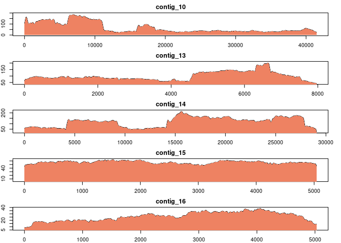
plotrange(myfiles, 6:10)
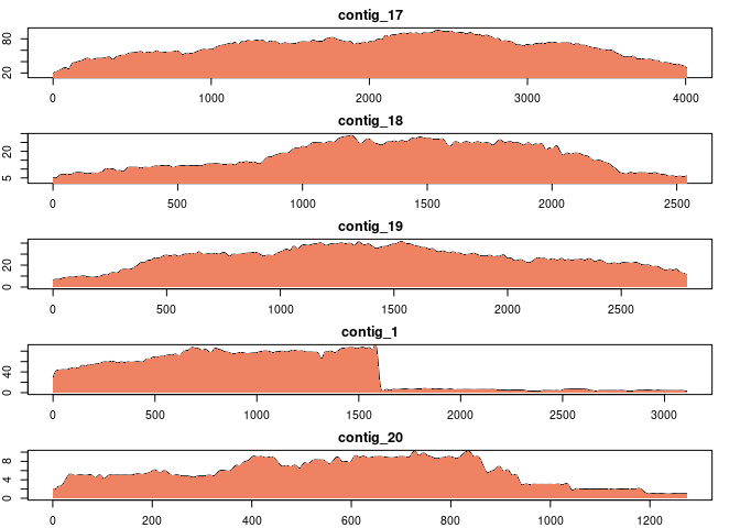
plotrange(myfiles, 11:15)
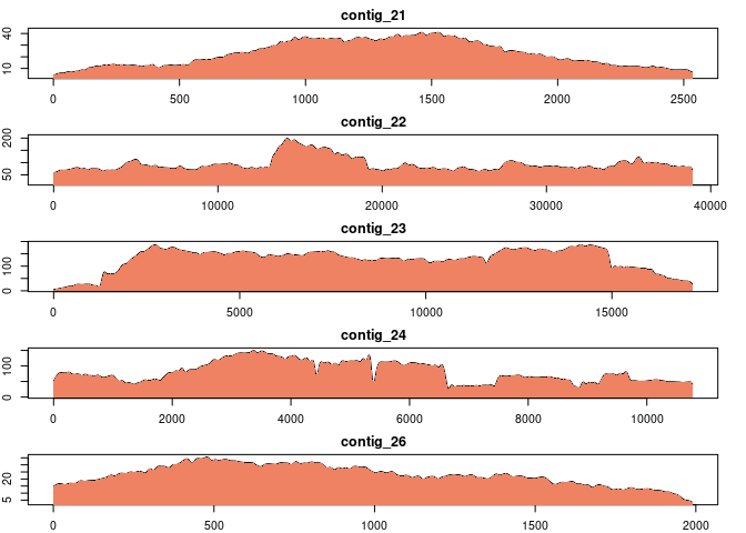
plotrange(myfiles, 16:20)
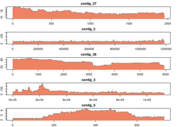
plotrange(myfiles, 21:25)
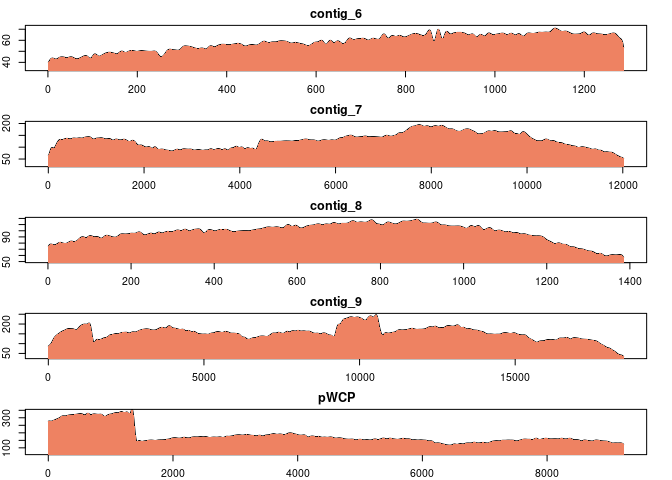
library(dplyr)
mndf <- data.frame(Column2 = character(), Column3 = numeric())
for (i in 1:length(myfiles)) {
    df <- myfiles[[i]]
    mn <- mean(df$V3, na.rm = TRUE)
    new_row <- data.frame(Column2 = contigs[[i]], Column3 = mn)
    mndf <- bind_rows(mndf, new_row)
}
#myfiles[[i]]$V2, myfiles[[i]]$V3, main=names(myfiles)[i])
head(mndf, 30L)
##      Column2    Column3
## 1  contig_10  65.230923
## 2  contig_13  98.625188
## 3  contig_14 116.216911
## 4  contig_15  55.992063
## 5  contig_16  26.009154
## 6  contig_17  66.010482
## 7  contig_18  17.126378
## 8  contig_19  26.840746
## 9   contig_1  39.219685
## 10 contig_20   5.629513
## 11 contig_21  22.494870
## 12 contig_22  92.771265
## 13 contig_23 127.043007
## 14 contig_24  80.674995
## 15 contig_26  22.833082
## 16 contig_27  16.875064
## 17  contig_2  31.022067
## 18 contig_38  60.132986
## 19  contig_3  50.671482
## 20  contig_5   5.528044
## 21  contig_6  58.553571
## 22  contig_7 129.096688
## 23  contig_8  97.561011
## 24  contig_9 156.366189
## 25      pWCP 183.192133
combined_df <- do.call(rbind, myfiles)
grouped_df <- combined_df %>% group_by(V1)
grouped_df
## # A tibble: 1,524,538 × 3
## # Groups:   V1 [25]
##    V1           V2    V3
##    <chr>     <int> <int>
##  1 contig_10     1    68
##  2 contig_10     2    71
##  3 contig_10     3    72
##  4 contig_10     4    73
##  5 contig_10     5    74
##  6 contig_10     6    75
##  7 contig_10     7    75
##  8 contig_10     8    75
##  9 contig_10     9    75
## 10 contig_10    10    76
## # ℹ 1,524,528 more rows
summary_df <- grouped_df %>%
  summarize(
    Median = median(V3, na.rm=TRUE),
    Mean = mean(V3, na.rm = TRUE),
    SD = sd(V3, na.rm = TRUE)
  )
summary_df
## # A tibble: 25 × 4
##    V1        Median  Mean    SD
##    <chr>      <dbl> <dbl> <dbl>
##  1 contig_1      44  39.2 34.6
##  2 contig_10     39  65.2 47.4
##  3 contig_13     89  98.6 33.2
##  4 contig_14    127 116.  44.7
##  5 contig_15     56  56.0  4.31
##  6 contig_16     27  26.0  7.00
##  7 contig_17     71  66.0 17.2
##  8 contig_18     17  17.1  7.44
##  9 contig_19     28  26.8  8.93
## 10 contig_2      30  31.0  9.16
## # ℹ 15 more rows
write.csv(summary_df,"contigcov_dataframe_unfiltered.csv", row.names = FALSE)
Coverage plots for our quality-filtered mappings
We now want to observe the coverage for our mappings filtered by mapping quality.
library(dplyr)
setwd('../../17_Coverage_filtered/')
temp <- list.files(pattern = glob2rx("Coverage*.txt"), full.names=T)
myfiles <- lapply(temp, read.table, skip = "#")
names(myfiles) <- temp
contigs <- lapply(names(myfiles), function(x) paste(strsplit(x, "_")[[1]][4:4], collapse = "_"))
contigs <- lapply(contigs, function(x) tools::file_path_sans_ext(tools::file_path_sans_ext(x)))
contigs <- lapply(contigs, function(x) paste0(substr(x, 1, 6), '_', substr(x, 7, nchar(x))))
contigs <- lapply(contigs, function(x) remove_trailing_underscores(x))
myfiles <- lapply(seq_along(myfiles), function(i) filter(myfiles[[i]], myfiles[[i]]$V1==contigs[i])) # plasmid
names(myfiles) <- contigs
library(cowplot)
library(ggplot2)

plotrange = function (myfiles, range) {
  myplots=list()

  par(mfrow = c(max(length(range), 5), 1), mar = rep(2, 4))

  for (i in range) {
     x <- myfiles[[i]]$V2
     y <- myfiles[[i]]$V3
     smoothed_spline <- smooth.spline(x, y, spar = 1e-5)  # Decrease spar for sharper edges
     smoothed_y <- predict(smoothed_spline, x)$y
     myplots[[i]] = plot(x, y, main=names(myfiles[i]), pch=8, cex=0.2, type='n')
     lines(x, smoothed_y, col = "black")
     polygon(c(x, rev(x)), c(smoothed_y, rep(0, length(x))), col = "skyblue", border = NA)
  }
}
i = 1
for (myfile in myfiles) {
  write.csv(myfile,paste0("QC_Contigs/", paste0(contigs[i],"_contigcov_dataframe.csv")))
  i = i + 1
}
plotrange(myfiles, 1:5)
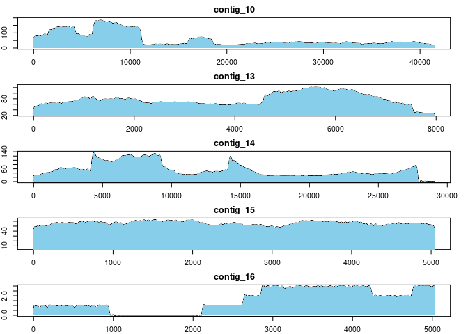
plotrange(myfiles, 6:10)
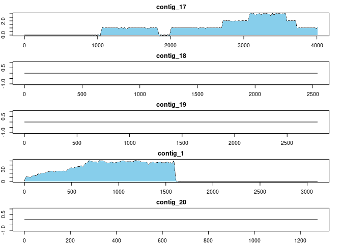
plotrange(myfiles, 11:15)
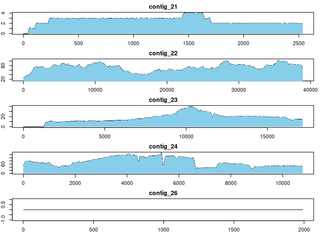
plotrange(myfiles, 16:20)
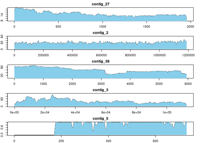
plotrange(myfiles, 21:25)
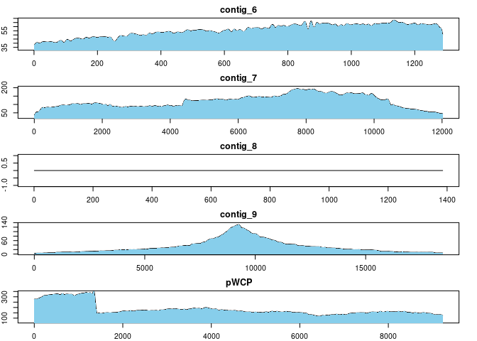
library(dplyr)
mndf <- data.frame(Column2 = character(), Column3 = numeric())
for (i in 1:length(myfiles)) {
    df <- myfiles[[i]]
    mn <- mean(df$V3, na.rm = TRUE)
    new_row <- data.frame(Column2 = contigs[[i]], Column3 = mn)
    mndf <- bind_rows(mndf, new_row)
}
#myfiles[[i]]$V2, myfiles[[i]]$V3, main=names(myfiles)[i])
head(mndf, 30L)
##      Column2     Column3
## 1  contig_10  59.0809605
## 2  contig_13  76.8991713
## 3  contig_14  54.6936128
## 4  contig_15  55.9920635
## 5  contig_16   1.5484577
## 6  contig_17   1.0611430
## 7  contig_18   0.0000000
## 8  contig_19   0.0000000
## 9   contig_1  19.3518816
## 10 contig_20   0.0000000
## 11 contig_21   2.5647198
## 12 contig_22  72.4334474
## 13 contig_23  17.0312937
## 14 contig_24  73.2308192
## 15 contig_26   0.0000000
## 16 contig_27  14.9134665
## 17  contig_2  29.6041165
## 18 contig_38  59.1259247
## 19  contig_3  41.2832900
## 20  contig_5   0.7277702
## 21  contig_6  55.6001553
## 22  contig_7 118.9592278
## 23  contig_8   0.0000000
## 24  contig_9  32.7499053
## 25      pWCP 183.1867143
combined_df <- do.call(rbind, myfiles)
grouped_df <- combined_df %>% group_by(V1)
grouped_df
## # A tibble: 1,524,538 × 3
## # Groups:   V1 [25]
##    V1           V2    V3
##    <chr>     <int> <int>
##  1 contig_10     1    59
##  2 contig_10     2    60
##  3 contig_10     3    61
##  4 contig_10     4    62
##  5 contig_10     5    63
##  6 contig_10     6    63
##  7 contig_10     7    63
##  8 contig_10     8    63
##  9 contig_10     9    63
## 10 contig_10    10    64
## # ℹ 1,524,528 more rows
summary_df <- grouped_df %>%
  summarize(
    Median = median(V3, na.rm=TRUE),
    Mean = mean(V3, na.rm = TRUE),
    SD = sd(V3, na.rm = TRUE)
  )
summary_df
## # A tibble: 25 × 4
##    V1        Median  Mean     SD
##    <chr>      <dbl> <dbl>  <dbl>
##  1 contig_1      11 19.4  21.0
##  2 contig_10     36 59.1  47.3
##  3 contig_13     70 76.9  22.6
##  4 contig_14     44 54.7  32.8
##  5 contig_15     56 56.0   4.31
##  6 contig_16      1  1.55  1.17
##  7 contig_17      1  1.06  0.957
##  8 contig_18      0  0     0
##  9 contig_19      0  0     0
## 10 contig_2      29 29.6   5.90
## # ℹ 15 more rows
write.csv(summary_df,"contigcov_dataframe_filtered.csv", row.names = FALSE)
Assessing the effect of MAPQ filtering
The ‘MAPQ < 2’ parameter removes all low-quality reads aligned with MAPQ 0 (some primary mappings and all secondary mappings) and with MAPQ 1 (some primary mappings).
Resources: https://github.com/lh3/minimap2/issues/447, https://www.biostars.org/p/9564847/
MAPQ filtering removes all minimap2 secondary mapping:
samtools view Celg3_SUP-Wolb_onlybac_corrected.bam | grep tp:A:S | head
a4979cfc-008b-4660-a9d9-15b67f00a537  256   contig_2    1   0   2297S66M1D2M1D112M1I38M1D72M2I7M1I54M1D18M1D4M1I62M1I38M1I140M3D5M2D1M1D67M3D107M2D8M1D37M1I202M1D46M1I10M1I104M1D109M1I15M1D268M1D59M2D9M1D215M1D493M2I88M3D117M2D113M2D155M6D4M2D5M1I27M  *   0   0   *   *   NM:i:95ms:i:5279    AS:i:5260   nn:i:0  tp:A:S  cm:i:417    s1:i:2483   de:f:0.0261 rl:i:0
b6b914b8-d3ca-4ad3-bdd0-a6009f0ecbd9    256 contig_2    1   0   5716S69M1I2M1D126M3I22M1I186M1I6M1I9M1D4M2D136M1I69M1I10M1I229M2D54M1D39M1I62M1D74M1I33M1D24M1D124M1I3M1I9M1I23M1D4M1D22M2I35M1S    *   0   0   *   *NM:i:50    ms:i:2472   AS:i:2468   nn:i:0  tp:A:S  cm:i:186    s1:i:1190   de:f:0.0322 rl:i:0
5d551fc1-fc37-4561-a473-d8b032cf7052    256 contig_2    1   0   2476S142M1D211M1I66M1I161M1D2M1D2M1D1M1D461M1I5M2D4M1I71M1I28M1D4M2D4M1D6M4I296M1I242M1I3M1I14M1I518M3D126M3I250M1D6M2D446M6S   *   0   0   *   *NM:i:51    ms:i:5882   AS:i:5872   nn:i:0  tp:A:S  cm:i:507    s1:i:2884   de:f:0.0133 rl:i:0
cab663fb-eb8c-4480-8a4d-e40ce9163554    256 contig_2    1   0   3922S21M1D43M2D2M1I2M1D148M1D27M1I138M1D202M3D299M4D181M6I7M2I34M1I160M2D4M1D59M1D32M2D40M1I91M1I8M1I9M1I376M2I645M1D10M1I43M1I63M1I14M1D48M2I9M2D8M1I7M2D361M1D23M3D15M2D16M9S *   0   0   *   *   NM:i:74 ms:i:5951   AS:i:5930   nn:i:0  tp:A:S  cm:i:492    s1:i:2819   de:f:0.0167 rl:i:0
dc76631e-4881-45f4-ab74-7948856c9a92    272 contig_2    1   0   2957S227M2D7M1D102M1D244M3I27M2D146M2I13M1D35M4D5M1I6M1I7M4D129M1D5M2I75M1D3M2D251M1I108M1D226M1D365M1S *   0   0   *   *   NM:i:46 ms:i:3751   AS:i:3738   nn:i:0  tp:A:S  cm:i:302    s1:i:1784   de:f:0.0165 rl:i:0
5d84a860-2d3f-46c9-b939-297f640ed62c    272 contig_2    1   0   5280S558M1D8M1I453M2I677M2D219M *   0   0   *   *   NM:i:12ms:i:3768    AS:i:3766   nn:i:0  tp:A:S  cm:i:325    s1:i:1849   de:f:0.0052 rl:i:0
7b88381b-05a4-431a-89e0-d7d7fd848725    256 contig_2    601 0   44S13M1D14M1I13M1D31M1I4M1D17M1D3M1I185M2I48M2I2M1D600M2D16M1D4M3D100M1I28M1I160M2D32M1D13M1D4M2I215M1D2M2I323M1D4M1I289M9S *   0   0   *   *NM:i:69    ms:i:1059   AS:i:3858   nn:i:0  tp:A:S  cm:i:331    s1:i:1848   de:f:0.0285 rl:i:0
2735ae7c-4d77-4217-84a2-3b88561d8cc7    272 contig_2    607 0   44S29M1I6M1D31M1I4M1D17M1D3M1I73M1I14M1D135M1I2M1D5M1I69M1I8M1D7M1I2M5I1M1D100M1I18M1D3M1D7M1D74M7D4M5D121M2I2M1I2M2D1M1D40M2D13M1I16M1D25M1I13M2D79M1D58M1I159M2D28M1I67M2I8M1I164M1I24M1I1M2I7M3D23M1D495M1D7M1D44M1S *   0   0   **  NM:i:152    ms:i:1129   AS:i:3198   nn:i:0  tp:A:S  cm:i:235s1:i:1419   de:f:0.0628 rl:i:0
2b7c47ea-7a4e-42c4-947d-95852de433a8    272 contig_2    715 0   83S103M1D6M1I177M1D50M1D13M2D3M1I5M1D24M1I7M2D2M2D14M1I21M1D13M2D11M1D23M1I13M1I4M4D11M2D9M1I124M1I1M3I241M1I5M2I59M1I16M1I8M1D52M5D5M2I14M1D2M3I10M1D7M1D56M   *0  0   *   *   NM:i:77 ms:i:822    AS:i:1828   nn:i:0  tp:A:S  cm:i:127    s1:i:798    de:f:0.0517 rl:i:0
7c52b5b1-84de-493a-b7ec-c3d822bb52ae    256 contig_2    749 0   5S74M4D2M1D11M2I5M1D20M1I20M23S *   0   0   *   *   NM:i:12ms:i:212 AS:i:208    nn:i:0  tp:A:S  cm:i:10 s1:i:85 de:f:0.0584 rl:i:0
samtools view Celg3_SUP-Wolb_onlybac_quality.bam | grep tp:A:S | head
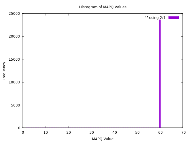
Here are the distributions of MAPQ values before and after filtering:
samtools view Celg3_SUP-Wolb_onlybac_corrected_sorted.bam | cut -f 5 | sort | uniq -c | gnuplot -p -e "
set title 'Histogram of MAPQ Values';
set xlabel 'MAPQ Value';
set ylabel 'Frequency';
set boxwidth 0.5;
set style fill solid;
plot '-' using 2:1 with boxes;"
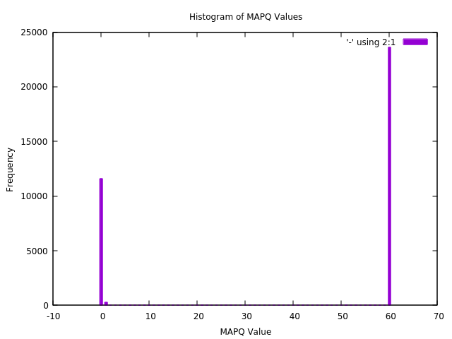
samtools view Celg3_SUP-Wolb_onlybac_quality_sorted.bam | cut -f 5 | sort | uniq -c | gnuplot -p -e "
set title 'Histogram of MAPQ Values';
set xlabel 'MAPQ Value';
set ylabel 'Frequency';
set boxwidth 0.5;
set style fill solid;
plot '-' using 2:1 with boxes;"