RosaBioinfo

Reproducible bioinformatic analyses for Tutagata et al.

Blandine Trouche 2024-07-16

• 1- Quality-filtering the raw data
• 2- Running Phyloflash to estimate eukaryotic vs bacterial proportion
  • 2a- Running PhyloFlash
  • 2b- Plotting taxonomic diversity at domain level
  • 2c- Plotting number of prokaryotic reads and phylotypes by sample
  • 2d- Plotting the prokaryotic diversity (Fig. 5A)
• 3- Genome reconstruction
  • 3a- Masking the Culex quinquefasciatus genome for short read removal
  • 3b- Running the snakemake metagenomic workflow
  • 3c- Refining the bins in the interactive interface
  • 3d- Dereplicating the MAGs and re-running the workflow for final read recruitment
  • 3e- Plotting the resulting coverage information (Fig. 5B)

The raw data is available on ENA under Bioproject ID: PRJEB77608
For the purpose of this bioinformatic workflow, the raw data was placed in folder RAW_DATA in the work datawork.

1- Quality-filtering the raw data

Let’s start by removing the adapters with bbduk.
We will need an adapter fasta file (here named scripts/adapter-seq.fa) containing the adapter sequence. You can copy and paste the following lines to create your own file.

>adapter_MGX  
CTGTCTCTTATACACATCT

Running bbduk:

# activate appropriate environment
conda activate bbmap-38.93

# creating output folders
mkdir -p 01_Trimmed 01_Trimmed/stats

for r1 in RAW_DATA/*_R1_001.fastq.gz
do

# copy the filename, r1, to a new file name, r2 and substitute R1 in the name with R2
# this generates the name of the R2 file
    r1=$(echo $r1 | sed 's|.*\/||')
    r2="${r1/_R1/_R2}"
    
# generate the names for the output files
    r1t="${r1/_R1_001.fastq.gz/_R1_trimmed.fastq.gz}"
    r2t="${r2/_R2_001.fastq.gz/_R2_trimmed.fastq.gz}"
    NAME="${r1/_R1_001.fastq.gz/}"
    echo "Name:$NAME"

# run bbduk
bbduk.sh  in1=RAW_DATA/$r1 in2=/RAW_DATA/$r2 \
          out1=01_Trimmed/$r1t out2=01_Trimmed/$r2t \
          ref=scripts/adapter-seq.fa \
          stats=01_Trimmed/stats/"$NAME"_stats.txt \
          ktrim=r k=19 mink=9 hdist=1 tpe tbo t=20 
done    
conda deactivate

Preparing the sample file for quality filtering through Anvi’o using Illumina-utils with Minoche quality filter:

for r1 in 01_Trimmed/*_R1_trimmed.fastq.gz; do
  r2="${r1/_R1/_R2}"
  r1short="${r1/01_Trimmed\//}"
  r1short="${r1short/_R1_trimmed.fastq.gz/}"
  echo -e "${r1short}\t${r1}\t${r2}" >> scripts/samples.txt
done

Running the first steps of the Anvi’o snakemake metagenomic workflow: quality filtering with Illumina-utils, zipping the resulting fastq files.
This was run on a high performance cluster (Migale), hence the cluster-specific parts of the command.
Config files are available in an archive on github for reproducibility.

conda activate anvio-7.1

anvi-run-workflow -w metagenomics -c config_QC.json \
                  --additional-params --until gzip_fastqs \
                  --cluster-config cluster.yml \
                  --cluster 'qsub -V -cwd -N {rule} -q {cluster.queue} -o {log} -e {log} -pe thread {threads}' \
                  --jobs 20 --jobscript jobscript.sh \
                  --rerun-incomplete --latency-wait 420

conda deactivate

Checking the results of quality filtering using FastQC and MultiQC

# running FastQC
conda activate fastqc-0.11.9
fastqc 01_QC_Trimmed/*.fastq.gz -o 01_QC_Trimmed/FastQC -t 25
conda deactivate 

# running MultiQC on FastQC results to aggregate them
conda activate multiqc-1.11 
multiqc 01_QC_Trimmed/FastQC -o 01_QC_Trimmed/MultiQC 
conda deactivate

2- Running Phyloflash to estimate eukaryotic vs bacterial proportion

2a- Running PhyloFlash

conda activate phyloflash-3.4.1

mkdir -p 02_Phyloflash
cd 02_Phyloflash

for r1 in ../01_QC_Trimmed/*_R1.fastq.gz
do
# copy the filename, r1, to a new file name, r2 and substitute R1 in the name with R2
# this generates the name of the R2 file
    r2="${r1/_R1/_R2}"
    NAME=$(echo $r1 | sed 's|.*\/||')
    NAME="${NAME/-QUALITY_PASSED_R1.fastq.gz/}"
    echo "Name:$NAME"

    mkdir -p $NAME
    
    phyloFlash.pl -lib ${NAME} -read1 ${r1} -read2 ${r2} \
                  -readlength 150 -almosteverything \
                  -CPUs 12 -dbhome /db/outils/phyloflash-3.4.1/138.1
done

conda deactivate

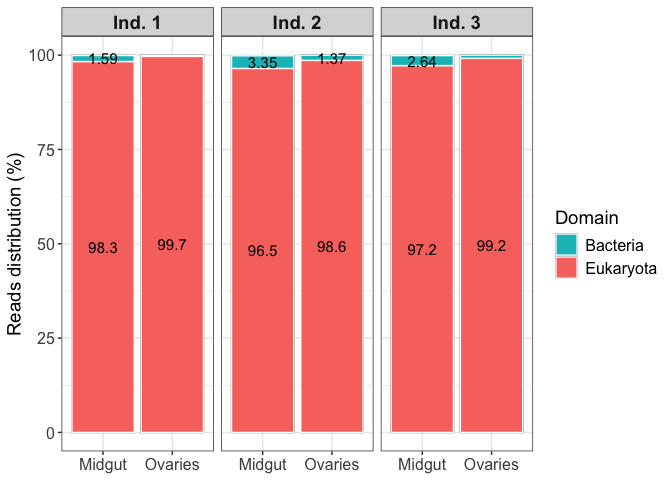
2b- Plotting taxonomic diversity at domain level

require(phyloseq)
require(data.table)
require(patchwork)
require(reshape2)
require(ggpubr)
require(svglite)
require(speedyseq)

# List of samples
samples <- list.files("02_Phyloflash")
samples <- samples[c(3:4, 13:16)]
# Initializing the full phylotype table
full_dt <- data.frame("Phylotype" = "NA")

# Reading each table and merging it with the previous ones
for (i in samples){
  NTU_table <- read.csv(paste0("02_Phyloflash/", 
                               i, "/", 
                               i, ".phyloFlash/", 
                               i, ".phyloFlash.NTUfull_abundance.csv"), 
                        header = FALSE)
  # renaming the columns
  colnames(NTU_table) <- c("Phylotype", i)
  
  # I want to have all samples in the same table so I will merge the phylotype tables
  full_dt <- merge(full_dt, NTU_table, by="Phylotype", all.x=TRUE, all.y=TRUE) 
}

# stats about the complete dataframe:
dim(full_dt)

## [1] 6197    7

full_dt[is.na(full_dt)] <- 0

#Number of phylotypes by sample
colSums(full_dt[2:ncol(full_dt)])

## NC014_VdC_Cxq_mg NC015_VdC_Cxq_ov NC046_VdC_Cxq_mg NC047_VdC_Cxq_ov 
##           458956           373507           275336           225122 
## NC054_VdC_Cxq_mg NC055_VdC_Cxq_ov 
##           291055           271690

For ease of plotting, I want to transform the data into a phyloseq object

# 1) creating the "otu table" aka the abundance table (columns 2 to end of datatable)
rownames(full_dt) <- paste0("Phylotype", c(1:nrow(full_dt)))
PHYLO <- full_dt[, c(2:ncol(full_dt))]
PHYLO <- otu_table(PHYLO, taxa_are_rows = TRUE)

# 2) creating the taxonomy table 
TAXO <- colsplit(full_dt$Phylotype, ";", c("Domain", "Phylum", "Class", "Order", "Family", "Genus", "Species"))
TAXO <- as.matrix(TAXO)
rownames(TAXO) <- rownames(full_dt)
TAXO <- tax_table(TAXO)

# 3) creating the metadata table
metadata <- data.frame(matrix(nrow = length(samples)))
rownames(metadata) <- samples

## general
metadata$Host <- "Culex quinquefasciatus"
metadata[grep('mg', rownames(metadata)), "Organ"] <- "Midgut"
metadata[grep('ov', rownames(metadata)), "Organ"] <- "Ovaries"

metadata$Individual <- c("Ind. 1", "Ind. 1", "Ind. 2", "Ind. 2", "Ind. 3", "Ind. 3")

## remove the first weird column
metadata <- metadata[, c(2:ncol(metadata))]
META <- sample_data(metadata)

# 4) creating the phyloseq object
ps_phylo <- phyloseq(PHYLO, TAXO, META)
rm(PHYLO, TAXO, META)

## making the phyloseq object relative abundance
ps_phylo_rel <- transform_sample_counts(ps_phylo, function(x) x / sum(x) * 100)

Plotting the repartition at domain level

# Archaea are not visible on the domain plot so let's remove them (as well as NA)
ps_phylo_rel_domain <- subset_taxa(ps_phylo_rel, Domain != "Archaea")
# aggregate by domain so it's pretty and fast
ps_phylo_rel_domain <- tax_glom(ps_phylo_rel_domain, taxrank = rank_names(ps_phylo_rel_domain)[1], NArm = FALSE)

# order Domain levels
domain_color = c("Eukaryota" = "#F8766D", "Bacteria" = "#00BFC4")

# plot
p1 <- plot_bar(ps_phylo_rel_domain, x = "Organ", fill = "Domain", facet_grid = ~Individual) + 
  geom_col(position = "stack", color="white") +
  labs(x = "Sample", y = "Reads distribution (%)", fill="Domain") +
  scale_fill_manual(values = domain_color) +
  geom_text(aes(label = ifelse(signif(Abundance, digits = 3) > 1, signif(Abundance, digits = 3), "")),
            position = position_stack(vjust = 0.5),
            color="black", size=4) +
  theme_bw() +
  theme(axis.text = element_text(size = 12), 
        axis.title.y = element_text(size = 14), 
        axis.title.x = element_blank(), 
        strip.text = element_text(face = "bold", size = 14), 
        legend.title = element_text(size = 14),
        legend.text = element_text(size = 12)) 
p1

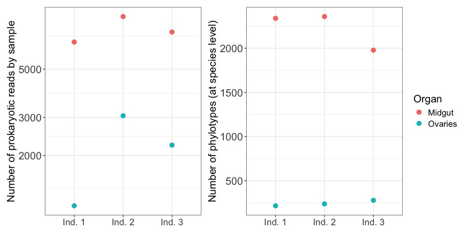
2c- Plotting number of prokaryotic reads and phylotypes by sample

# We now focus only on Bacteria and Archaea
ps_phylo_prok <- subset_taxa(ps_phylo, Domain != "Eukaryota")
# also remove mitochondria and chloroplast
ps_phylo_prok <- subset_taxa(ps_phylo_prok, Family != "Mitochondria")
ps_phylo_prok <- subset_taxa(ps_phylo_prok, Order != "Chloroplast")

phylo_nb <- ps_phylo_prok@sam_data

# adding to the dataframe the number of reads by sample
phylo_nb$Total_reads <- sample_sums(ps_phylo_prok)

# adding to the dataframe the number of taxa by sample
phylo_nb$Nb_phylo <- apply(ps_phylo_prok@otu_table > 0, 2, sum)

# Number of reads by method
nb_reads <- ggplot(phylo_nb, aes(x = Individual, y = Total_reads)) +
  geom_point(aes(color = Organ), size = 3) +  
  theme_bw() +
  theme(axis.title.x=element_blank(),
        axis.text.x=element_text(size = 14),
        axis.text.y = element_text(face="plain",size=16),
        axis.title.y = element_text(size=16),
        legend.text = element_text(size=13),
        legend.title = element_text(size=16),
        strip.text.x = element_text(size = 14)) +
  ylab("Number of prokaryotic reads by sample") + scale_y_log10()

# Number of phylotypes by method
nb_phylo <- ggplot(phylo_nb, aes(x = Individual, y = Nb_phylo)) +
  geom_point(aes(color = Organ), size = 3) +
  theme_bw() +
  theme(axis.title.x=element_blank(),
        axis.text.x=element_text(size = 14),
        axis.text.y = element_text(face="plain",size=16),
        axis.title.y = element_text(size=16),
        legend.text = element_text(size=13),
        legend.title = element_text(size=16),
        strip.text.x = element_text(size = 14)) +
  ylab("Number of phylotypes (at species level)") 

nb_reads + nb_phylo +
  plot_layout(guides = 'collect')

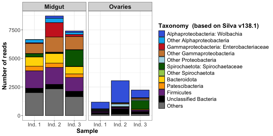
2d- Plotting the prokaryotic diversity (Fig. 5A)

ps_phylo_prok_rel <- ps_phylo_prok

# before agglomerating, let's try to remove affiliation that does not mean anything ()
ps_phylo_prok_rel@tax_table[grep("^\\(", ps_phylo_prok_rel@tax_table[,2]), 2] <- NA
ps_phylo_prok_rel@tax_table[grep("^\\(", ps_phylo_prok_rel@tax_table[,3]), 3] <- NA
ps_phylo_prok_rel@tax_table[grep("^\\(", ps_phylo_prok_rel@tax_table[,4]), 4] <- NA
ps_phylo_prok_rel@tax_table[grep("^\\(", ps_phylo_prok_rel@tax_table[,5]), 5] <- NA
ps_phylo_prok_rel@tax_table[grep("^\\(", ps_phylo_prok_rel@tax_table[,6]), 6] <- NA
ps_phylo_prok_rel@tax_table[grep("^\\(", ps_phylo_prok_rel@tax_table[,7]), 7] <- NA

general_taxo_phy <- speedyseq::tax_glom(ps_phylo_prok_rel, 
                                        taxrank=rank_names(ps_phylo_prok_rel)[2],
                                        NArm=FALSE)

df_phy <- data.frame(general_taxo_phy@tax_table[, c(1:2)]) # put same number as for tax_glom
df_phy$number_of_reads <- signif((taxa_sums(general_taxo_phy) / sum(taxa_sums(general_taxo_phy)) * 100), 3)
df_phy <- df_phy[order(-df_phy$number_of_reads),]

# choose how many to keep
phylum_to_keep <- df_phy$Phylum[1:6]

# keep chosen phylotypes and group the rest in "Others"
ps_phylo_prok_rel@tax_table[(ps_phylo_prok_rel@tax_table[,2] %in% phylum_to_keep) == FALSE,] <- "Others"

# aggregate again for ease of plotting
ps_phylo_prok_rel <- speedyseq::tax_glom(ps_phylo_prok_rel, 
                                         taxrank = rank_names(ps_phylo_prok_rel)[6], 
                                         NArm = FALSE)

# more resolution as needed
taxo <- as.data.table(data.frame(ps_phylo_prok_rel@tax_table))

## diverse phyla
taxo[is.na(Phylum), Taxonomy:="Unclassified Bacteria"]
taxo[Phylum=="Others", Taxonomy:="Others"]
taxo[Phylum=="Bacteroidota", Taxonomy:="Bacteroidota"]
taxo[Phylum=="Patescibacteria", Taxonomy:="Patescibacteria"]
taxo[Phylum=="Firmicutes", Taxonomy:="Firmicutes"]

## proteobac
taxo[Family=="Enterobacteriaceae", Taxonomy:="Gammaproteobacteria: Enterobacteriaceae"]
taxo[Family=="Spirochaetaceae", Taxonomy:="Spirochaetota: Spirochaetaceae"]
taxo[Genus=="Wolbachia", Taxonomy:="Alphaproteobacteria: Wolbachia"]
taxo[Class=="Alphaproteobacteria" & is.na(Taxonomy), Taxonomy:="Other Alphaproteobacteria"]
taxo[Class=="Gammaproteobacteria" & is.na(Taxonomy), Taxonomy:="Other Gammaproteobacteria"]
taxo[Phylum=="Proteobacteria" & is.na(Taxonomy), Taxonomy:="Other Proteobacteria"]
taxo[Phylum=="Spirochaetota" & is.na(Taxonomy), Taxonomy:="Other Spirochaetota"]

setcolorder(taxo, neworder = c("Taxonomy", "Domain", "Phylum", "Class", "Order",
                               "Family", "Genus", "Species"))
            
taxo <- as.matrix(taxo)
rownames(taxo) <- taxa_names(ps_phylo_prok_rel)

ps_phylo_prok_rel <- phyloseq(otu_table(ps_phylo_prok_rel), tax_table(taxo), sample_data(ps_phylo_prok_rel))

test <- tax_glom(ps_phylo_prok_rel, taxrank = rank_names(ps_phylo_prok_rel)[1], 
                 NArm = TRUE)

physeqdf <- psmelt(test)
physeqdf$Taxonomy <- factor(physeqdf$Taxonomy,
                            levels = c("Alphaproteobacteria: Wolbachia", "Other Alphaproteobacteria",
                                       "Gammaproteobacteria: Enterobacteriaceae", "Other Gammaproteobacteria",
                                       "Other Proteobacteria", "Spirochaetota: Spirochaetaceae", 
                                       "Other Spirochaetota", "Bacteroidota",
                                       "Patescibacteria", "Firmicutes",
                                       "Unclassified Bacteria", "Others"))

# specifically defined color scale
scale_taxon = c("Alphaproteobacteria: Wolbachia" = "royalblue", 
                "Other Alphaproteobacteria" = "deepskyblue2",   
                "Gammaproteobacteria: Enterobacteriaceae" = "firebrick3", 
                "Other Gammaproteobacteria" = "tan3",
                "Other Proteobacteria" = "lightblue", 
                "Spirochaetota: Spirochaetaceae" = "darkgreen", 
                "Other Spirochaetota" = "darkolivegreen3", 
                "Bacteroidota" = "gold", "Patescibacteria" = "orange", 
                "Firmicutes" = "mediumorchid4", "Unclassified Bacteria" = "black", 
                "Others" = "grey50")

p4 <- ggplot(physeqdf, aes(x = Individual, y = Abundance, fill = Taxonomy)) +
  facet_grid(~Organ) +
  geom_bar(stat = "identity", position = "stack", color = "black") +
  labs(x = "Sample", y = "Number of reads", 
       fill="Taxonomy  (based on Silva v138.1)", color="Taxonomy  (based on Silva v138.1)") +
  scale_color_manual(values = scale_taxon) +
  scale_fill_manual(values = scale_taxon) +
  theme_bw() +
  theme(axis.text = element_text(size = 14, angle = 0), 
        axis.title = element_text(size = 16, face = "bold"), 
        strip.text = element_text(face = "bold", size = 16), 
        legend.text = element_text(size = 14), 
        legend.title = element_text(size = 16, face = "bold")) 
p4 

svg("Export_figures/Figure1A.svg", width=10, height=6)
p4
dev.off()

## quartz_off_screen 
##                 2

3- Genome reconstruction

3a- Masking the Culex quinquefasciatus genome for short read removal

Culex quinquefasciatus accession: GCF_015732765.1
wPipPel accession: GCF_000073005.1

# activate conda environment
conda activate bbmap-38.93

ref_folder=00_Ref_data
wPipPel_folder=$ref_folder/01_FASTA/wPipPel

# make output folder
mkdir -p $ref_folder/Cxq_masked

# unzip ref genomes 
gunzip $ref_folder/Culex_quinquefasciatus-contigs.fa.gz
gunzip $wPipPel_folder/wPipPel.fa.gz

# use bbmask to mask the Culex quinque genome and avoid future problems when removing it by mapping
# 1) prepare wPipPel for mapping
shred.sh in=$wPipPel_folder/wPipPel.fa \
    out=$ref_folder/Cxq_masked/wPipPel-contigs_shredded.fa \
    length=80 minlength=70 overlap=40

# 2) map Culex to wPipPel to identify similar sequences
bbmap.sh ref=$ref_folder/Culex_quinquefasciatus-contigs.fa \
        in=$ref_folder/Cxq_masked/wPipPel-contigs_shredded.fa \
        outm=$ref_folder/Cxq_masked/Cxq_to_wPipPel_mapped.sam \
    minid=0.85 maxindel=2 \
    threads=6

# 3) mask similar sequences, zones with low entropy and tandem-repeated kmers
bbmask.sh in=$ref_folder/Culex_quinquefasciatus-contigs.fa \
        out=$ref_folder/Cxq_masked/Cxq_masked.fa \
        entropy=0.7 sam=$ref_folder/Cxq_masked/Cxq_to_wPipPel_mapped.sam \
        threads=6

gzip $ref_folder/*.fa
gzip $wPipPel_folder/*.fa

# deactivate conda environment
conda deactivate

3b- Running the snakemake metagenomic workflow

# create the samples file for the metagenomic workflow (post-QC)
for r1 in 01_QC_Trimmed/*-QUALITY_PASSED_R1.fastq.gz; do
  r2="${r1/_R1/_R2}"
  r1short="${r1/01_QC_Trimmed\//}"
  r1short="${r1short/-QUALITY_PASSED_R1.fastq.gz/}"
  echo -e "${r1short}\t${r1}\t${r2}" >> scripts/QC_samples.txt
done

# run the workflow, including the removal of short reads based on the Culex quinquefasciatus genome
conda activate anvio-7.1

anvi-run-workflow -w metagenomics -c config_megahit_JOVE.json \
    --additional-params --cluster-config cluster.yml \
    --cluster 'qsub -V -cwd -N {rule} -q {cluster.queue} -o {log} -e {log} -pe thread {threads}' \
    --jobs 10 --jobscript jobscript.sh --rerun-incomplete --latency-wait 420

# deactivate conda environment
conda deactivate

Following the workflow, we bin contigs using CONCOCT, restricting the number of bins created to 3:

# binning contigs
for sample in NC014_VdC_Cxq_mg_noCulex NC015_VdC_Cxq_ov_noCulex \
              NC046_VdC_Cxq_mg_noCulex NC047_VdC_Cxq_ov_noCulex \
              NC054_VdC_Cxq_mg_noCulex NC055_VdC_Cxq_ov_noCulex 
do
    anvi-cluster-contigs -p 06_MERGED/${sample}/PROFILE.db \
                     -c 03_CONTIGS/${sample}-contigs.db \
                     -C CONCOCT_3 --driver CONCOCT \
                     --clusters 3 \
                     --just-do-it >> 00_LOGS/anvi-cluster-contigs_concoct3_${sample}.log  
done

# summarizing the bins to obtain info before refining
for sample in NC014_VdC_Cxq_mg_noCulex NC015_VdC_Cxq_ov_noCulex \
              NC046_VdC_Cxq_mg_noCulex NC047_VdC_Cxq_ov_noCulex \
              NC054_VdC_Cxq_mg_noCulex NC055_VdC_Cxq_ov_noCulex 
do
    anvi-summarize -p 06_MERGED/${sample}/PROFILE.db \
               -c 03_CONTIGS/${sample}-contigs.db \
               -o 07_SUMMARY/${sample} \
               -C CONCOCT_3   
done

3c- Refining the bins in the interactive interface

# examples of refining commands
anvi-refine -p 06_MERGED/NC014_VdC_Cxq_mg_noCulex/PROFILE.db \
    -c 03_CONTIGS/NC014_VdC_Cxq_mg_noCulex-contigs.db \
    -C CONCOCT_3 -b Bin_2

anvi-refine -p 06_MERGED/NC054_VdC_Cxq_mg_noCulex/PROFILE.db \
    -c 03_CONTIGS/NC054_VdC_Cxq_mg_noCulex-contigs.db \
    -C CONCOCT_3 -b Bin_2 

# summarizing the results of refinment to obtain the final information about the MAGs
for sample in NC014_VdC_Cxq_mg_noCulex NC015_VdC_Cxq_ov_noCulex \
              NC046_VdC_Cxq_mg_noCulex NC047_VdC_Cxq_ov_noCulex \
              NC054_VdC_Cxq_mg_noCulex NC055_VdC_Cxq_ov_noCulex
do
    anvi-summarize -p 06_MERGED/${sample}/PROFILE.db \
               -c 03_CONTIGS/${sample}-contigs.db \
               -o 08_SUMMARY_refined/${sample} \
               -C CONCOCT_3   
done

3d- Dereplicating the MAGs and re-running the workflow for final read recruitment

conda activate anvio-7.1 

# creating the genome file for dereplication
# It can be done by Anvi'o automatically as outlined below.
# Here I have chosen to prepare the file by hand to include only bins of interest (over 0.8 completion and 1 Mbp long), and to make their names more explicit 

#for sample in NC014_VdC_Cxq_mg_noCulex NC015_VdC_Cxq_ov_noCulex \
#              NC046_VdC_Cxq_mg_noCulex NC047_VdC_Cxq_ov_noCulex \
#              NC054_VdC_Cxq_mg_noCulex NC055_VdC_Cxq_ov_noCulex
#do
#anvi-script-gen-genomes-file -c 03_CONTIGS/${sample}-contigs.db \
#          -p 06_MERGED/${sample}/PROFILE.db \
#          -C CONCOCT_3 \
#          -o bins_for_derep_${sample}.txt
#done

# dereplicating the genomes based on pyANI
anvi-dereplicate-genomes --internal-genomes scripts/bins_for_derep.txt \
          --output-dir 10_DEREP \
          --program pyANI \
          --min-alignment-fraction 0.7 \
          --similarity-threshold 0.99 \
          --representative-method length \
          --log-file 00_LOGS/anvi-dereplicate-genomes.log
# length used instead of Qscore because of an error in code. It was fixed in Anvi'o dev in 02/2024

# concatenate the cluster representative MAGs for mapping onto
mkdir -p 10_DEREP/02_FASTA
cat 10_DEREP/GENOMES/*.fa > 10_DEREP/02_FASTA/Ref_MAGS.fa

# the fasta file is made by hand and available in the archive
# generating the samples file
for r1 in 01_QC/*-FILTERED_R1.fastq.gz; do
  r2="${r1/_R1/_R2}"
  r1short="${r1/01_QC\//}"
  r1short="${r1short/-FILTERED_R1.fastq.gz/}"
  echo -e "${r1short}\t${r1}\t${r2}" >> scripts/noCulex_samples.txt
done

# run workflow in reference mode to obtain final mapping (done locally)
anvi-run-workflow -w metagenomics \
          -c mapping_JOVE_config.json \
          --additional-params --rerun-incomplete --keep-going
          
# extract contig names from MAGs to make a collection to reimport in new database
while read line; do
 echo -e "${line}\tNC014_Bin_2_1_BR149"
done < 08_SUMMARY_refined/NC014_VdC_Cxq_mg_noCulex/bin_by_bin/Bin_2_1/Bin_2_1-original_split_names.txt \
      > 10_DEREP/02_FASTA/NC014_mg_Bin_2_1_split.txt

while read line; do
 echo -e "${line}\tNC046_Bin_1_1_1_Entero"
done < ../08_SUMMARY_refined/NC046_VdC_Cxq_mg_noCulex/bin_by_bin/Bin_1_1_1/Bin_1_1_1-original_split_names.txt \
      > 10_DEREP/02_FASTA/NC046_Bin_1_1_1_split.txt

while read line; do
 echo -e "${line}\tNC054_Bin_2_1_Pantoea"
done < ../08_SUMMARY_refined/NC054_VdC_Cxq_mg_noCulex/bin_by_bin/Bin_2_1/Bin_2_1-original_split_names.txt \
      > 10_DEREP/02_FASTA/NC054_Bin_2_1_split.txt

while read line; do
 echo -e "${line}\tNC055_Bin_2_1_Wolbachia"
done < ../08_SUMMARY_refined/NC055_VdC_Cxq_ov_noCulex/bin_by_bin/Bin_2_1/Bin_2_1-original_split_names.txt \
      > 10_DEREP/02_FASTA/NC055_Bin_2_1_split.txt

cat 10_DEREP/02_FASTA/*_split.txt > Ref_MAGs_collection.txt

cd 10_DEREP

anvi-import-collection Ref_MAGs_collection.txt \
                       -c 03_CONTIGS/Ref_MAGs-contigs.db \
                       -p 06_MERGED/Ref_MAGs/PROFILE.db \
                       -C Ref_MAGs

anvi-summarize -p 06_MERGED/Ref_MAGs/PROFILE.db \
               -c 03_CONTIGS/Ref_MAGs-contigs.db \
               -o 07_SUMMARY \
               -C Ref_MAGs

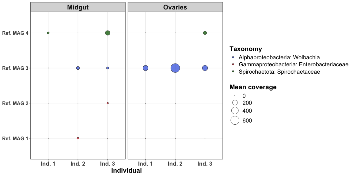
3e- Plotting the resulting coverage information (Fig. 5B)

require(tidyr)
require(dplyr)

df_mean <- data.frame()
df_detec <- data.frame()

# read dataframes
df_mean <- read.table("10_DEREP/07_SUMMARY/bins_across_samples/mean_coverage.txt", header = TRUE)
df_mean_long <- pivot_longer(df_mean, cols = c(2:ncol(df_mean)))
colnames(df_mean_long) <- c( "bins", "metagenome", "mean_coverage")

df_detec <- read.table("10_DEREP/07_SUMMARY/bins_across_samples/detection.txt", header = TRUE)
df_detec_long <- pivot_longer(df_detec, cols = c(2:ncol(df_detec)))
colnames(df_detec_long) <- c( "bins", "metagenome", "detection")

df <- full_join(df_detec_long, df_mean_long)

# coverage = 0 if detection < 0.9
df[df$detection < 0.9, "mean_coverage"] <- 0
df[grep("mg", df$metagenome), "Organ"] <- "Midgut"
df[grep("ov", df$metagenome), "Organ"] <- "Ovaries"

# add taxonomy similar to Phyloflash
df[df$bins == "NC046_Bin_1_1_1_Entero" | df$bins == "NC054_Bin_2_1_Pantoea",
   "Taxonomy"] <- "Gammaproteobacteria: Enterobacteriaceae"
df[df$bins == "NC055_Bin_2_1_Wolbachia", "Taxonomy"] <- "Alphaproteobacteria: Wolbachia"
df[df$bins == "NC014_Bin_2_1_BR149", "Taxonomy"] <- "Spirochaetota: Spirochaetaceae"

# add individual
df[df$metagenome == "NC014_mg_noCulex" | df$metagenome == "NC015_ov_noCulex",
   "Individual"] <- "Ind. 1"
df[df$metagenome == "NC046_mg" | df$metagenome == "NC047_ov",
   "Individual"] <- "Ind. 2"
df[df$metagenome == "NC054_mg_noCulex" | df$metagenome == "NC055_ov_noCulex",
   "Individual"] <- "Ind. 3"

# change MAG name
df[df$bins == "NC046_Bin_1_1_1_Entero", "MAG"] <- "Ref. MAG 1"
df[df$bins == "NC054_Bin_2_1_Pantoea", "MAG"] <- "Ref. MAG 2"
df[df$bins == "NC055_Bin_2_1_Wolbachia", "MAG"] <- "Ref. MAG 3"
df[df$bins == "NC014_Bin_2_1_BR149", "MAG"] <- "Ref. MAG 4"

# color
df$Taxonomy <- factor(df$Taxonomy,
                      levels = c("Alphaproteobacteria: Wolbachia",
                                 "Gammaproteobacteria: Enterobacteriaceae",
                                 "Spirochaetota: Spirochaetaceae"))

# specifically defined color scale
scale_taxonomy = c("Alphaproteobacteria: Wolbachia" = "royalblue", 
                "Gammaproteobacteria: Enterobacteriaceae" = "firebrick3", 
                "Spirochaetota: Spirochaetaceae" = "darkgreen")

# plot
p1 <- ggplot(df, aes(x = MAG, y = Individual)) +
  facet_grid(~Organ) +
  geom_point(aes(size = mean_coverage, fill = Taxonomy), 
             alpha = 0.75, shape = 21) +
  scale_size(range = c(.1, 10), name="Mean coverage") + 
  scale_fill_manual(values = scale_taxonomy) +
  theme_bw() +
  theme(axis.text.x = element_text(face = "bold", size = 14),
        axis.text.y = element_text(face = "bold", size = 12),
        strip.text = element_text(face = "bold", size = 16), 
        axis.title.x = element_text(size = 16, face = "bold"),
        axis.title.y = element_blank(),
        legend.text = element_text(size = 14), 
        legend.title = element_text(size = 16, face = "bold")) +
  coord_flip()
p1

# export as svg to refine in your favorite graphic editor
svg("Export_figures/Figure1B.svg", width=10, height=6)
p1  
dev.off()

## quartz_off_screen 
##                 2