RosaBioinfo
Quantitative analysis of WO phage induction assays
January 26, 2026
Alice Brunner
Language: R
Notebook setup
Packages
# Packages

library(ggplot2)
library(readxl)
library(ggpubr)
library(lme4)
library(emmeans)
library(DHARMa)
library(performance)
library(tidyr)
Data
The following files: Data/induction_slab_results.xlsx and Data/induction_mito_slab_R_results.xlsx are required.
# Data

Temp_data <- read_excel('Data/induction_slab_results.xlsx')

Mito_data <- read_excel('Data/induction_mito_slab_R_results.xlsx')
Temperature treatment
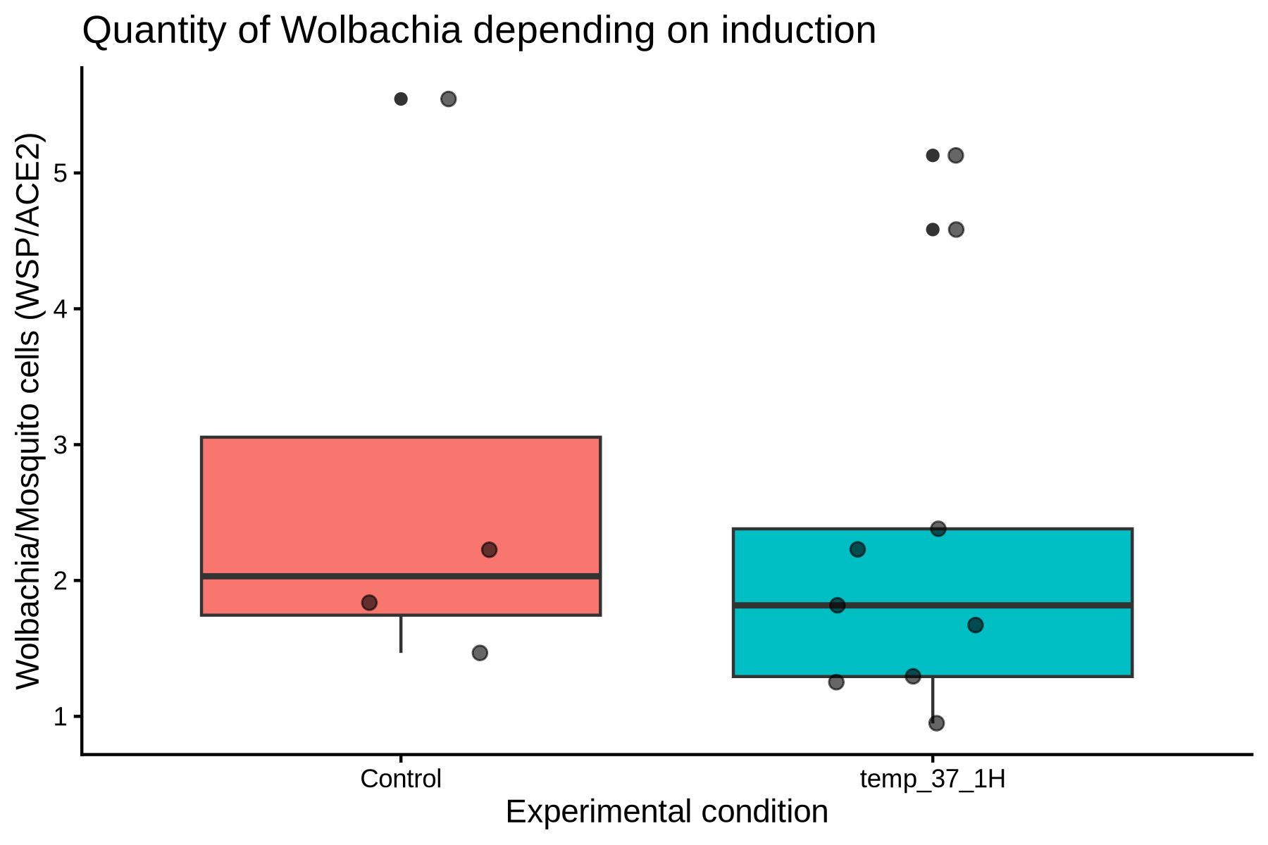
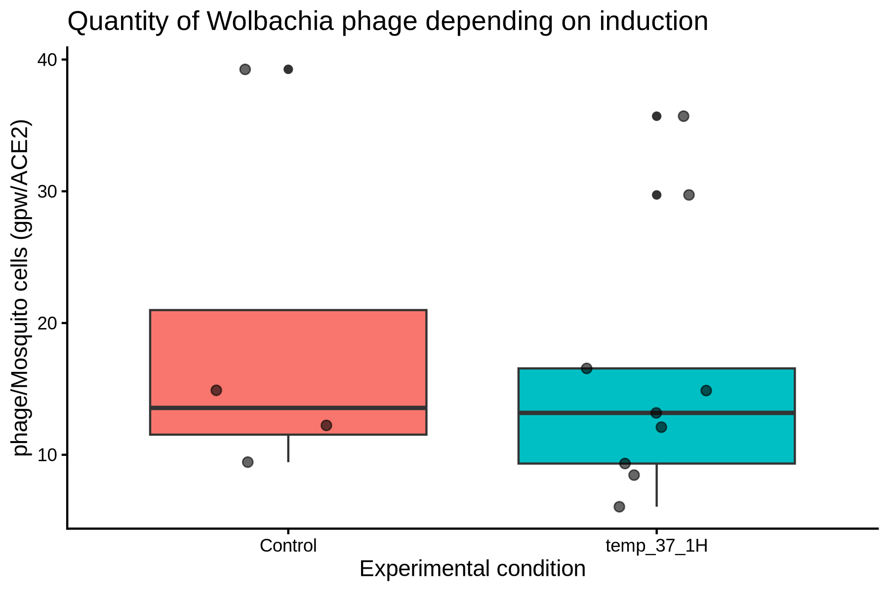
This section presents the qPCR-based quantification of Wolbachia and WO phage abundance following thermal induction of adult SLAB females. Statistical comparisons between treated and control groups were performed using Wilcoxon rank-sum tests.
Plot on Wolbachia
#  Transformation de la variable "statut" en facteur avec un ordre spécifique
Temp_data$statut <- factor(Temp_data$type_induction, levels = c("temp_37_1H", "Control"))

#  Création d’un boxplot pour visualiser la quantité de *Wolbachia*
ggplot(Temp_data, aes(x = type_induction, y = wsp_ace2, fill = type_induction)) +
  geom_boxplot() +
  geom_jitter(position = position_jitter(0.2), size = 2, alpha = 0.6, color = "black") +
  theme_classic() +
  labs(title = "Quantity of Wolbachia depending on induction",
       x = "Experimental condition",
       y = "Wolbachia/Mosquito cells (WSP/ACE2)") +
  theme(legend.position = "none")
ggsave(
  filename = "Output/Figure_3B_1_wsp_temperature.png",
  width = 6, height = 4, dpi = 300
)
Plot on Phage WO
#  Plot WO

ggplot(Temp_data, aes(x = type_induction, y = gpw_ace2, fill = type_induction)) +
  geom_boxplot() +
  geom_jitter(position = position_jitter(0.2), size = 2, alpha = 0.6, color = "black") +
  theme_classic() +
  labs(title = "Quantity of Wolbachia phage depending on induction",
       x = "Experimental condition",
       y = "phage/Mosquito cells (gpw/ACE2)") +
  theme(legend.position = "none")
ggsave(
  filename = "Output/Figure_3B_1_WO_temperature.png",
  width = 6, height = 4, dpi = 300
)
Stats on Wolbachia
wilcox_wsp <- wilcox.test(
  wsp_ace2 ~ type_induction,
  data = Temp_data,
  exact = FALSE
)

wilcox_wsp
##
##  Wilcoxon rank sum test with continuity correction
##
## data:  wsp_ace2 by type_induction
## W = 22, p-value = 0.5892
## alternative hypothesis: true location shift is not equal to 0
Stats on Phage
wilcox_gpw <- wilcox.test(
  gpw_ace2 ~ type_induction,
  data = Temp_data,
  exact = FALSE
)

wilcox_gpw
##
##  Wilcoxon rank sum test with continuity correction
##
## data:  gpw_ace2 by type_induction
## W = 22, p-value = 0.5892
## alternative hypothesis: true location shift is not equal to 0
Mitomycine treatment
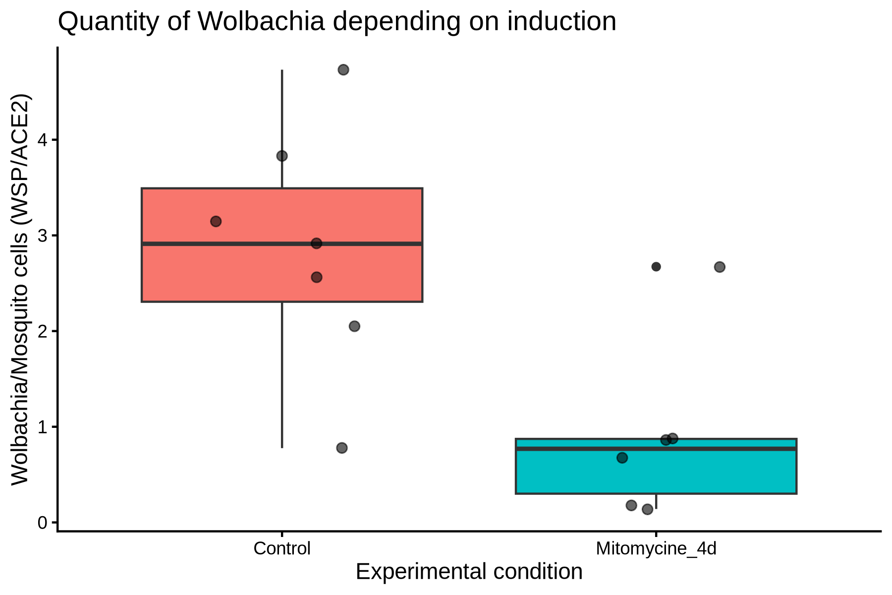
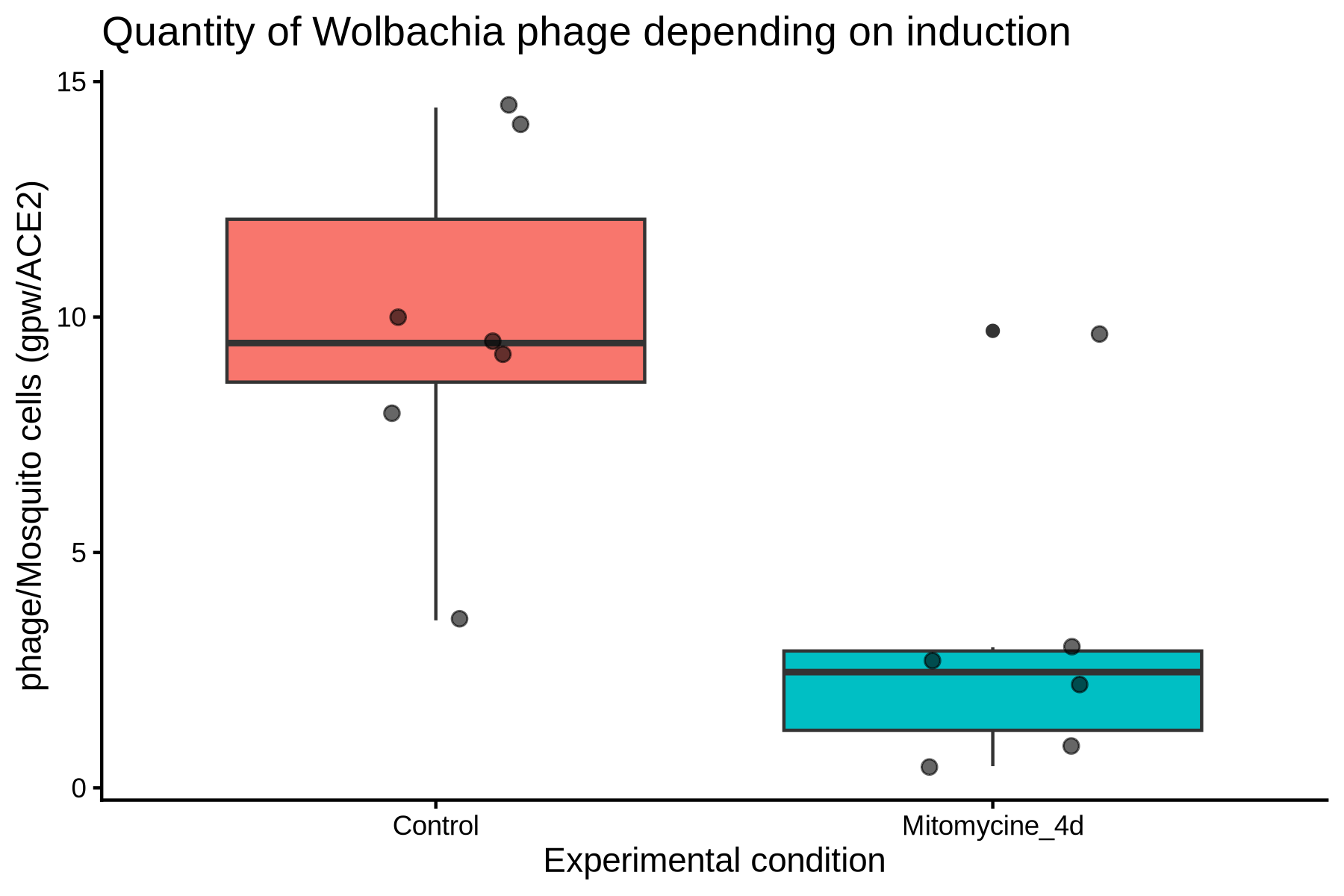
This section presents qPCR quantifications following chemical induction of first-instar SLAB larvae exposed to mitomycin C (5 ng ml⁻¹) for four days.
Plot on Wolbachia
Mito_data$statut <- factor(Mito_data$type_induction, levels = c("Mitomycine_4d", "Control"))

ggplot(Mito_data, aes(x = type_induction, y = wsp_ace2, fill = type_induction)) +
  geom_boxplot() +
  geom_jitter(position = position_jitter(0.2), size = 2, alpha = 0.6, color = "black") +
  theme_classic() +
  labs(title = "Quantity of Wolbachia depending on induction",
       x = "Experimental condition",
       y = "Wolbachia/Mosquito cells (WSP/ACE2)") +
  theme(legend.position = "none")
ggsave(
  filename = "Output/Figure_3B_2_Wolbachia_temperature.png",
  width = 6, height = 4, dpi = 300
)
Plot on Phage WO
ggplot(Mito_data, aes(x = type_induction, y = gpw_ace2, fill = type_induction)) +
  geom_boxplot() +
  geom_jitter(position = position_jitter(0.2), size = 2, alpha = 0.6, color = "black") +
  theme_classic() +
  labs(title = "Quantity of Wolbachia phage depending on induction",
       x = "Experimental condition",
       y = "phage/Mosquito cells (gpw/ACE2)") +
  theme(legend.position = "none")
ggsave(
  filename = "Output/Figure_3B_2_WO_temperature.png",
  width = 6, height = 4, dpi = 300
)
Stats on Wolbachia
wilcox_wsp <- wilcox.test(
  wsp_ace2 ~ type_induction,
  data = Mito_data,
  exact = FALSE
)

wilcox_wsp
##
##  Wilcoxon rank sum test with continuity correction
##
## data:  wsp_ace2 by type_induction
## W = 37, p-value = 0.02681
## alternative hypothesis: true location shift is not equal to 0
Stats on Phage quantities
wilcox_gpw <- wilcox.test(
  gpw_ace2 ~ type_induction,
  data = Mito_data,
  exact = FALSE
)

wilcox_gpw
##
##  Wilcoxon rank sum test with continuity correction
##
## data:  gpw_ace2 by type_induction
## W = 38, p-value = 0.01842
## alternative hypothesis: true location shift is not equal to 0