RosaBioinfo

Anvi’o pangenomic analyzes using pWCP, WO, wPipSLAB and wPipPel including addition of metagenomic data layers

January 7, 2026

Maxime Mahout

Notebook for creation and annotation of an anvi’o pangenome

Language: Bash

Contigs database creation

anvi-script-reformat-fasta final-Wolbachia-contigs.fa --simplify-names -o formatted-Wolbachia-contigs.fa

anvi-gen-contigs-database -f formatted-Wolbachia-contigs.fa -o Isolate1-contigs.db

anvi-get-sequences-for-gene-calls -c Isolate1-contigs.db --export-gff3 -o Isolate1-genes.gff

anvi-get-sequences-for-gene-calls -c Isolate1-contigs.db --get-aa-sequences -o PROTEINS.fa

Pangenome creation

cat Data/external_genomes_latest.csv

## name contigs_db_path
## WOPip1   ../Phages/WOPip1-contigs.db
## WOPip2   ../Phages/WOPip2-contigs.db
## WOPip3   ../Phages/WOPip3-contigs.db
## WOPip4   ../Phages/WOPip4-contigs.db
## WOPip5   ../Phages/WOPip5-contigs.db
## wPipPel   ../PipRef/wPipPel-contigs.db
## pWCP ../PipRef/pWCP-contigs.db
## wPipSLAB  ./wSLAB002o-contigs.db
## Isolate1 ./Isolate1-contigs.db

anvi-gen-genomes-storage -e external_genomes_latest.csv -o ISOLATE-GENOMES.db

anvi-pan-genome --mcl-inflation 10 --use-ncbi-blast -g ISOLATE-GENOMES.db -n ISOLATE_PAN -T 4

Display pangenome and remove outliers

We display the generated pangenome using the following command:

anvi-display-pan -p ISOLATE_PAN/ISOLATE_PAN-PAN.db -g ISOLATE-GENOMES.db

The resulting pangenome contains 1143 GCs (Gene Clusters).

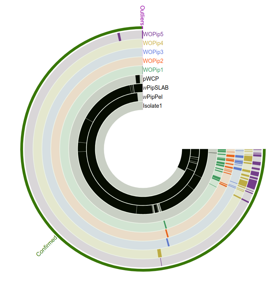
In the following steps we want to extract all GCs, detect where the cif genes are located, and indicate single copy genes.

However, we need to remove two outlier GCs, that appear as two erroneous Prodigal gene calls on WO FASTA files, given that WO are extracted from wPipPel and should contain the same information.

We checked where those two GCs are located in wPipPel, and they are located in intergenic regions, indicating that these are likely not really genes.

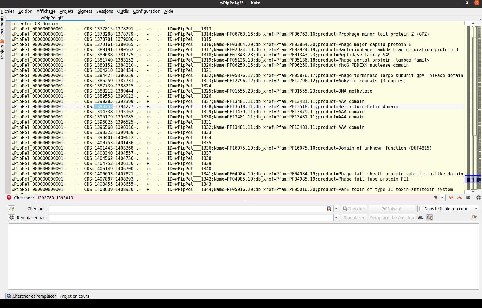
Note how the detected WO gene region in the search bar is between two genes in wPipPel.gff and therefore intergenic.

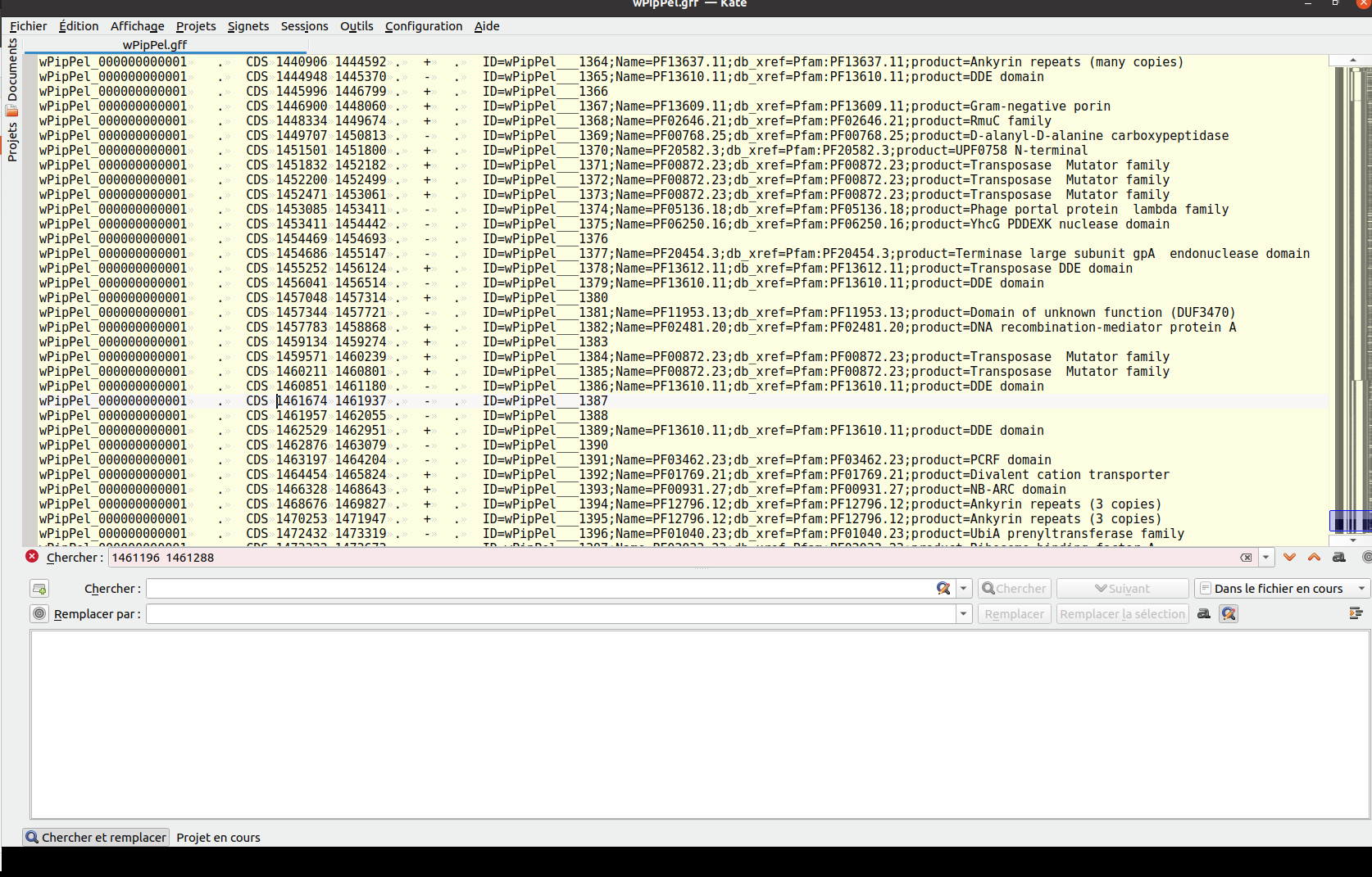
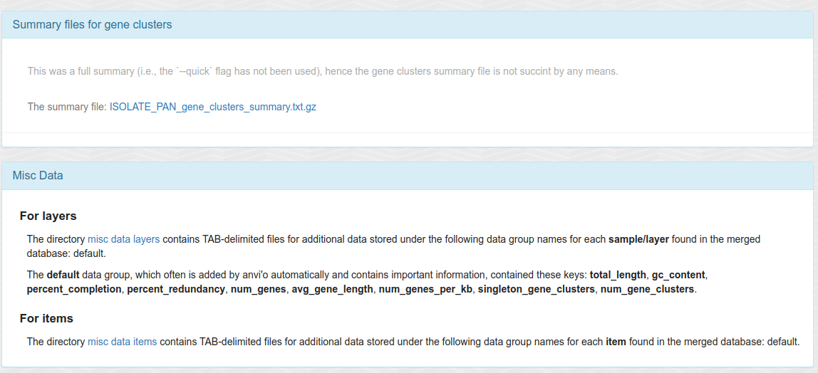
Having two bins (namely “Confirmed”, “Outliers”) allow us to make a summary of the GCs (ISOLATE_PAN_gene_clusters_summary.txt), which we will use in the Notebook 4 (Python) to extract gene information.

For the rest of the analyzes and especially the main figures and main text, we will exclude the two Outliers and work with 1141 GCs.

Mapping SLAB and Isolate on SLAB assembly

As detaled in previous Notebooks, SLAB assembly does not contain Culex contigs as Culex reads were depleted.

bowtie2-align-s --wrapper basic-0 --threads 4 -x ./SLAB002_Cxq_ov-contigs --passthrough -1 ./SLAB002_Cxq_ov-FILTERED_R1.fastq.gz -2 ./SLAB002_Cxq_ov-FILTERED_R2.fastq.gz > SLAB002_Cxq_ov.bam

bowtie2-align-s --wrapper basic-0 --threads 4 -x ./SLAB002_Cxq_ov-contigs --passthrough -1 ./Isolate1-FILTERED_R1.fastq.gz -2 ./Isolate1-FILTERED_R2.fastq.gz > Isolate1_FILTERED.bam

Both short read pairs are aligned to SLAB002 assembly (from which we extract wPipSLAB) with bowtie.

Preparing coverage for the pangenome

Coverage on wPipSLAB is calculated with bedtools genomecov.

bedtools genomecov -d -ibam SLAB002_Cxq_ov.bam > Coverage_SLAB002_Cxq_ov.txt

bedtools genomecov -d -ibam Isolate1_FILTERED.bam > Coverage_Isolate1-FILTERED.txt

Filter only contigs of SLAB002 that correspond to Wolbachia (wPipSLAB).

grep ">" SLAB002_Cxq_ov/Wolbachia-contigs.fa | sed 's/^>//' > SLAB_Wolbachia_contigs.fa

Now get the coverage correspond to those contigs (reads mapping to wPipSLAB):

grep -F -f SLAB_Wolbachia_contigs.fa Coverage_SLAB002_Cxq_ov.txt > Coverage_SLAB002_Cxq_ov_filtered.txt

grep -F -f SLAB_Wolbachia_contigs.fa Coverage_Isolate1-FILTERED.txt > Coverage_Isolate1-FILTERED_filtered.txt

This gives us coverage files such as the following:

head Data/Coverage_SLAB002_Cxq_ov_filtered.txt -n 12

## SLAB002_Cxq_ov_000000000871  1   65
## SLAB002_Cxq_ov_000000000871  2   91
## SLAB002_Cxq_ov_000000000871  3   100
## SLAB002_Cxq_ov_000000000871  4   100
## SLAB002_Cxq_ov_000000000871  5   102
## SLAB002_Cxq_ov_000000000871  6   102
## SLAB002_Cxq_ov_000000000871  7   102
## SLAB002_Cxq_ov_000000000871  8   103
## SLAB002_Cxq_ov_000000000871  9   105
## SLAB002_Cxq_ov_000000000871  10  112
## SLAB002_Cxq_ov_000000000871  11  134
## SLAB002_Cxq_ov_000000000871  12  138

head Data/Coverage_Isolate1-FILTERED_filtered.txt -n 12

## SLAB002_Cxq_ov_000000000871  1   0
## SLAB002_Cxq_ov_000000000871  2   0
## SLAB002_Cxq_ov_000000000871  3   0
## SLAB002_Cxq_ov_000000000871  4   4
## SLAB002_Cxq_ov_000000000871  5   4
## SLAB002_Cxq_ov_000000000871  6   4
## SLAB002_Cxq_ov_000000000871  7   8
## SLAB002_Cxq_ov_000000000871  8   8
## SLAB002_Cxq_ov_000000000871  9   8
## SLAB002_Cxq_ov_000000000871  10  8
## SLAB002_Cxq_ov_000000000871  11  8
## SLAB002_Cxq_ov_000000000871  12  8

Download these files here: Coverage_SLAB002_Cxq_ov_filtered.txt and Coverage_Isolate1-FILTERED_filtered.txt.

Anvio commands for preparing Python notebook analysis

Export items data for getting number of genome hits in particular

anvi-export-misc-data --target-data-table items -p ISOLATE_PAN/ISOLATE_PAN-PAN.db -o ISOLATE_PAN_ITEMS.tsv

This is useful in generating the layer of the pangenome for single copy genes.

Get the GFF of wPipSLAB for gene coverage calculation

anvi-get-sequences-for-gene-calls -c ./wSLAB002o-contigs.db --export-gff -o wSLAB002o.gff --annotation-source Pfam

The GFF of SLAB contains prodigal gene calling IDs.

However, we will also need to associated those gene calling IDs with their corresponding pangenome gene cluster IDs.

Generate a FASTA of all gene clusters which header contains gene calling IDs

anvi-get-sequences-for-gene-clusters -g ISOLATE-GENOMES.db -p ISOLATE_PAN/ISOLATE_PAN-PAN.db --report-DNA-sequences -o ISOLATE_PAN_GENE_CLUSTERS.fasta --max-num-genomes-gene-cluster-occurs 100 --max-num-genes-from-each-genome 100

Now we can go on with the Jupyter Python Notebook 4.

Adding coverage to the pangenome

anvi-import-misc-data --target-data-table items -p ISOLATE_PAN/ISOLATE_PAN-PAN.db ISOLATE_PAN_ITEMS_Isolate1_SLAB_against_SLAB.tsv

Using the file ISOLATE_PAN_ITEMS_Isolate1_SLAB_against_SLAB.tsv generated by the Notebook 4.

Splitting pangenome to remove outliers and display split pangenome

anvi-split -p ISOLATE_PAN/ISOLATE_PAN-PAN.db -o ISOLATE_PAN/Confirmed -g ISOLATE-GENOMES.db -b Confirmed -C default

anvi-display-pan -p ISOLATE_PAN/Confirmed/Confirmed/PAN.db -g ISOLATE-GENOMES.db -P 8080

Or, if we want to simply show the full pangenome

anvi-display-pan -p ISOLATE_PAN/ISOLATE_PAN-PAN.db -g ISOLATE-GENOMES.db -P 8080