RosaBioinfo
Inter-stage statistics of expression of pWCP genes in Wolbachia endosymbiont of Culex using RT-qPCR concentrations
Mateo Jarry
2026-01-22
Data loading
This notebook needs in input “Data/Culex_SLAB_design.xlsx” (get here).
library(readxl)
library(ggplot2)
data <- read_excel('./Data/Culex_SLAB_design.xlsx', sheet = 'R_data_expression')
str(data)
## tibble [2,310 × 5] (S3: tbl_df/tbl/data.frame)
##  $ ID_tube           : chr [1:2310] "SLAB_F_1" "SLAB_F_2" "SLAB_F_3" "SLAB_F_4" ...
##  $ Stage             : chr [1:2310] "Female" "Female" "Female" "Female" ...
##  $ Plate             : chr [1:2310] "qPCR_MJ1" "qPCR_MJ1" "qPCR_MJ1" "qPCR_MJ1" ...
##  $ GENE              : chr [1:2310] "wsp" "wsp" "wsp" "wsp" ...
##  $ Concentration Mean: chr [1:2310] "9.7399999999999999E-8" "1.801E-7" "1.4999999999999999E-7" "4.2E-7" ...
data$GENE <- as.factor(data$GENE)
data$Plate <- as.factor(data$Plate)
data$Stage <- as.factor(data$Stage)
data$concentration <- as.numeric(data$`Concentration Mean`)
## Warning: NAs introduced by coercion
data_cleaned <- na.omit(data)
data_cleaned <- data.frame(data_cleaned)
summary(data_cleaned)
##    ID_tube             Stage           Plate                 GENE
##  Length:2258        Female:330   qPCR_MJ1 :  88   Dnab-1 (GP02): 207
##  Class :character   L1    :287   qPCR_MJ10:  88   RelB_1       : 207
##  Mode  :character   L2    :322   qPCR_MJ11:  88   RelE_2       : 207
##                     L3    :329   qPCR_MJ12:  88   Dnab-2 (GP02): 206
##                     L4    :330   qPCR_MJ14:  88   GP09         : 206
##                     Male  :330   qPCR_MJ15:  88   RelB_2       : 206
##                     Nymph :330   (Other)  :1730   (Other)      :1019
##  Concentration.Mean concentration
##  Length:2258        Min.   :2.100e-10
##  Class :character   1st Qu.:7.464e-08
##  Mode  :character   Median :5.360e-07
##                     Mean   :2.459e-06
##                     3rd Qu.:2.105e-06
##                     Max.   :1.750e-04
##
Data sorting and cleaning
library(dplyr)
##
## Attaching package: 'dplyr'

## The following objects are masked from 'package:stats':
##
##     filter, lag

## The following objects are masked from 'package:base':
##
##     intersect, setdiff, setequal, union
# Filter dataset for Male stage
data_male <- data_cleaned %>% filter(Stage == "Male")

data_female <- data_cleaned %>% filter(Stage == "Female")

# Deletion of a female F12 (anormaly high cDNA concentration)
data_withoutF12 <- data_female %>% filter(ID_tube != "SLAB_F_12")

data_nymph <- data_cleaned %>% filter(Stage == "Nymph")

data_L4 <- data_cleaned %>% filter(Stage == "L4")

# Deletion of a female L4_24 (anormaly high cDNA concentration)

data_withoutL4_24 <- data_L4 %>% filter(ID_tube != "SLAB_L4_24")

data_L3 <- data_cleaned %>% filter(Stage == "L3")

data_L2 <- data_cleaned %>% filter(Stage == "L2")

data_L1 <- data_cleaned %>% filter(Stage == "L1")

# Add a 'Stage' column to each dataset
data_male$Stage <- "Male"
data_female$Stage <- "Female"
data_nymph$Stage <- "Nymph"
data_L4$Stage <- "L4"
data_L3$Stage <- "L3"
data_L2$Stage <- "L2"
data_L1$Stage <- "L1"

# Fuse the datasets
data_combined <- bind_rows(data_L1, data_L2, data_L3, data_withoutL4_24, data_nymph, data_male, data_withoutF12)
Interstage analyses
Boxplot inter-stages for the 11 genes with kruskal test (for each gene)
library(ggpubr)

ggboxplot(
  data_combined,
  x = "Stage",
  y = "concentration",
  color = "Stage",
  facet.by = "GENE",
  scales = "free_y"
) +
  stat_compare_means(
    method = "kruskal.test",
    label = "p.format",        # or "p.signif" for stars
    label.y.npc = 0.95,        # 95% up from the bottom (inside the panel)
    size = 4                   # tweak text size if needed
  ) +
  scale_y_log10() +
  theme(
    axis.title.x = element_blank(),
    axis.text.x  = element_blank(),
    axis.ticks.x = element_blank()
  )
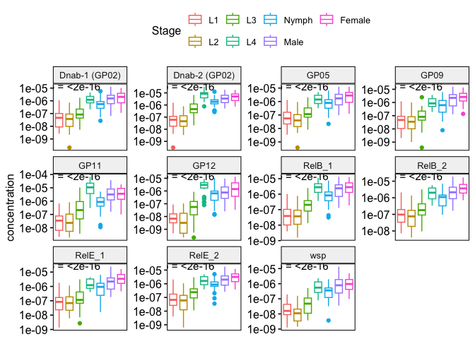
# Ccl: Each gene is showing at least one significant difference between two stage for every genes
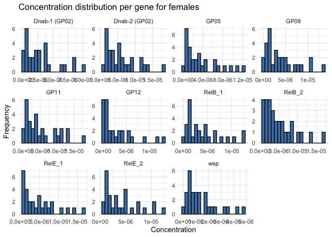
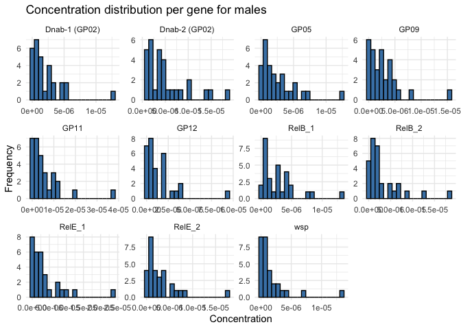
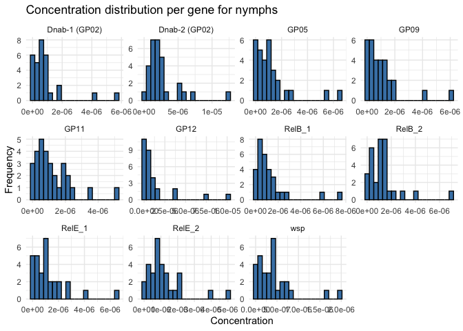
cDNA concentration distribution per gene
Females
ggplot(data_withoutF12, aes(x = concentration)) +
  geom_histogram(bins = 20, fill = "steelblue", color = "black") +
  facet_wrap(~ GENE, scales = "free") +
  theme_minimal() +
  labs(title = "Concentration distribution per gene for females",
       x = "Concentration",
       y = "Frequency")
Males
ggplot(data_male, aes(x = concentration)) +
  geom_histogram(bins = 20, fill = "steelblue", color = "black") +
  facet_wrap(~ GENE, scales = "free") +
  theme_minimal() +
  labs(title = "Concentration distribution per gene for males",
       x = "Concentration",
       y = "Frequency")
Nymphs
ggplot(data_nymph, aes(x = concentration)) +
  geom_histogram(bins = 20, fill = "steelblue", color = "black") +
  facet_wrap(~ GENE, scales = "free") +
  theme_minimal() +
  labs(title = "Concentration distribution per gene for nymphs",
       x = "Concentration",
       y = "Frequency")
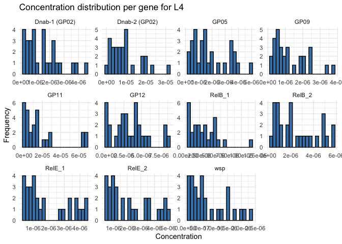
L4
ggplot(data_withoutL4_24, aes(x = concentration)) +
  geom_histogram(bins = 20, fill = "steelblue", color = "black") +
  facet_wrap(~ GENE, scales = "free") +
  theme_minimal() +
  labs(title = "Concentration distribution per gene for L4",
       x = "Concentration",
       y = "Frequency")
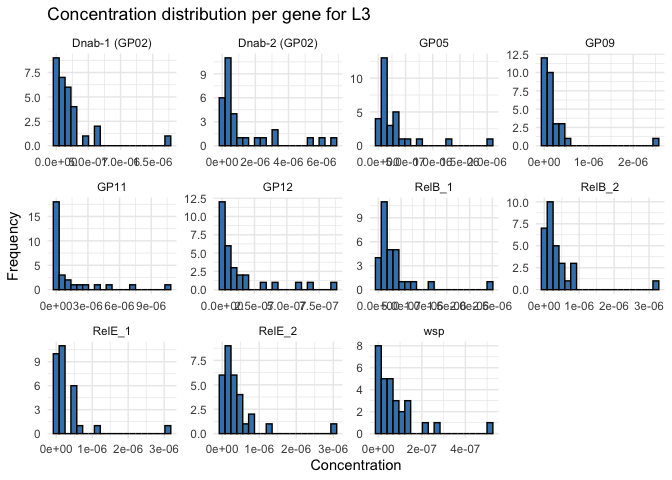
L3
ggplot(data_L3, aes(x = concentration)) +
  geom_histogram(bins = 20, fill = "steelblue", color = "black") +
  facet_wrap(~ GENE, scales = "free") +
  theme_minimal() +
  labs(title = "Concentration distribution per gene for L3",
       x = "Concentration",
       y = "Frequency")
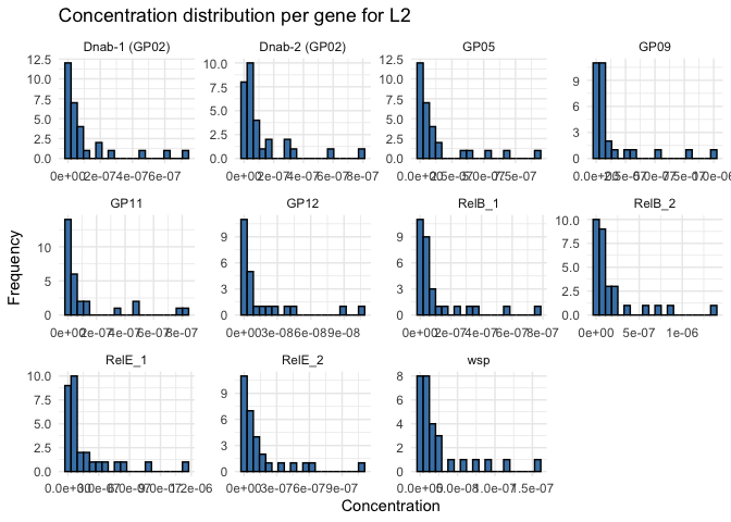
L2
ggplot(data_L2, aes(x = concentration)) +
  geom_histogram(bins = 20, fill = "steelblue", color = "black") +
  facet_wrap(~ GENE, scales = "free") +
  theme_minimal() +
  labs(title = "Concentration distribution per gene for L2",
       x = "Concentration",
       y = "Frequency")
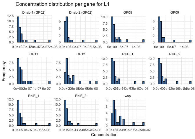
L1
ggplot(data_L1, aes(x = concentration)) +
  geom_histogram(bins = 20, fill = "steelblue", color = "black") +
  facet_wrap(~ GENE, scales = "free") +
  theme_minimal() +
  labs(title = "Concentration distribution per gene for L1",
       x = "Concentration",
       y = "Frequency")
GLMM with qPCR plate as random effect term
library(emmeans)
## Warning: package 'emmeans' was built under R version 4.3.3

## Welcome to emmeans.
## Caution: You lose important information if you filter this package's results.
## See '? untidy'
library(glmmTMB)
## Warning in checkDepPackageVersion(dep_pkg = "TMB"): Package version inconsistency detected.
## glmmTMB was built with TMB version 1.9.10
## Current TMB version is 1.9.11
## Please re-install glmmTMB from source or restore original 'TMB' package (see '?reinstalling' for more information)
# List of genes
genes <- unique(data_combined$GENE)

# Create a list to stock results
results_glmm <- list()

# Adjust GLMM model for the gene
for (gene in genes) {

  # Filter the data for this gene
  data_gene <- subset(data_combined, GENE == gene)

  # Adjust GLMM model for the gene
  model_glmm <- glmmTMB(concentration ~ Stage + (1 | Plate),
                        data = data_gene,
                        family = Gamma(link = "log"))

  # Extract post-hoc comparisons results
  emm_glmm <- emmeans(model_glmm, ~ Stage)
  post_hoc_glmm <- pairs(emm_glmm, adjust = "Bonferroni")

  # Stocker the results
  results_glmm[[gene]] <- post_hoc_glmm
}

# Display the results for one specific gene
print(results_glmm[["Dnab-1 (GP02)"]])
##  contrast       estimate    SE  df z.ratio p.value
##  Female - L1      2.8051 0.600 Inf   4.678  0.0001
##  Female - L2      4.2474 0.586 Inf   7.250  <.0001
##  Female - L3      2.3987 0.599 Inf   4.005  0.0013
##  Female - L4      0.7050 0.581 Inf   1.213  1.0000
##  Female - Male    0.5096 0.494 Inf   1.032  1.0000
##  Female - Nymph   0.6931 0.576 Inf   1.203  1.0000
##  L1 - L2          1.4423 0.567 Inf   2.543  0.2311
##  L1 - L3         -0.4064 0.588 Inf  -0.691  1.0000
##  L1 - L4         -2.1002 0.598 Inf  -3.513  0.0093
##  L1 - Male       -2.2955 0.591 Inf  -3.883  0.0022
##  L1 - Nymph      -2.1121 0.562 Inf  -3.758  0.0036
##  L2 - L3         -1.8488 0.591 Inf  -3.126  0.0372
##  L2 - L4         -3.5425 0.594 Inf  -5.962  <.0001
##  L2 - Male       -3.7378 0.565 Inf  -6.611  <.0001
##  L2 - Nymph      -3.5544 0.624 Inf  -5.692  <.0001
##  L3 - L4         -1.6937 0.598 Inf  -2.831  0.0975
##  L3 - Male       -1.8890 0.589 Inf  -3.207  0.0282
##  L3 - Nymph      -1.7056 0.570 Inf  -2.990  0.0586
##  L4 - Male       -0.1953 0.561 Inf  -0.348  1.0000
##  L4 - Nymph      -0.0119 0.523 Inf  -0.023  1.0000
##  Male - Nymph     0.1834 0.541 Inf   0.339  1.0000
##
## Results are given on the log (not the response) scale.
## P value adjustment: bonferroni method for 21 tests
print(results_glmm[["Dnab-2 (GP02)"]])
##  contrast       estimate    SE  df z.ratio p.value
##  Female - L1       3.324 0.541 Inf   6.150  <.0001
##  Female - L2       4.760 0.523 Inf   9.101  <.0001
##  Female - L3       1.762 0.537 Inf   3.278  0.0220
##  Female - L4      -0.325 0.525 Inf  -0.620  1.0000
##  Female - Male     0.400 0.444 Inf   0.899  1.0000
##  Female - Nymph    0.248 0.506 Inf   0.490  1.0000
##  L1 - L2           1.436 0.485 Inf   2.960  0.0646
##  L1 - L3          -1.563 0.530 Inf  -2.951  0.0665
##  L1 - L4          -3.650 0.543 Inf  -6.723  <.0001
##  L1 - Male        -2.925 0.524 Inf  -5.583  <.0001
##  L1 - Nymph       -3.076 0.505 Inf  -6.096  <.0001
##  L2 - L3          -2.999 0.500 Inf  -5.996  <.0001
##  L2 - L4          -5.086 0.521 Inf  -9.755  <.0001
##  L2 - Male        -4.361 0.501 Inf  -8.711  <.0001
##  L2 - Nymph       -4.512 0.533 Inf  -8.469  <.0001
##  L3 - L4          -2.087 0.539 Inf  -3.874  0.0023
##  L3 - Male        -1.362 0.519 Inf  -2.622  0.1836
##  L3 - Nymph       -1.514 0.512 Inf  -2.954  0.0659
##  L4 - Male         0.725 0.496 Inf   1.463  1.0000
##  L4 - Nymph        0.573 0.458 Inf   1.252  1.0000
##  Male - Nymph     -0.152 0.454 Inf  -0.334  1.0000
##
## Results are given on the log (not the response) scale.
## P value adjustment: bonferroni method for 21 tests
print(results_glmm[["GP05"]])
##  contrast       estimate    SE  df z.ratio p.value
##  Female - L1      2.7177 0.600 Inf   4.527  0.0001
##  Female - L2      4.3925 0.571 Inf   7.686  <.0001
##  Female - L3      2.3225 0.574 Inf   4.044  0.0011
##  Female - L4      0.6996 0.563 Inf   1.243  1.0000
##  Female - Male    0.6146 0.475 Inf   1.293  1.0000
##  Female - Nymph   0.6355 0.557 Inf   1.141  1.0000
##  L1 - L2          1.6748 0.596 Inf   2.811  0.1036
##  L1 - L3         -0.3952 0.581 Inf  -0.680  1.0000
##  L1 - L4         -2.0181 0.592 Inf  -3.406  0.0138
##  L1 - Male       -2.1031 0.595 Inf  -3.537  0.0085
##  L1 - Nymph      -2.0822 0.548 Inf  -3.799  0.0031
##  L2 - L3         -2.0700 0.557 Inf  -3.714  0.0043
##  L2 - L4         -3.6929 0.583 Inf  -6.336  <.0001
##  L2 - Male       -3.7779 0.549 Inf  -6.880  <.0001
##  L2 - Nymph      -3.7570 0.614 Inf  -6.121  <.0001
##  L3 - L4         -1.6229 0.573 Inf  -2.834  0.0967
##  L3 - Male       -1.7079 0.563 Inf  -3.035  0.0506
##  L3 - Nymph      -1.6870 0.554 Inf  -3.043  0.0491
##  L4 - Male       -0.0850 0.542 Inf  -0.157  1.0000
##  L4 - Nymph      -0.0641 0.499 Inf  -0.129  1.0000
##  Male - Nymph     0.0209 0.521 Inf   0.040  1.0000
##
## Results are given on the log (not the response) scale.
## P value adjustment: bonferroni method for 21 tests
print(results_glmm[["GP09"]])
##  contrast       estimate    SE  df z.ratio p.value
##  Female - L1       3.159 0.581 Inf   5.439  <.0001
##  Female - L2       4.437 0.571 Inf   7.772  <.0001
##  Female - L3       2.838 0.562 Inf   5.047  <.0001
##  Female - L4       1.190 0.555 Inf   2.145  0.6703
##  Female - Male     0.570 0.491 Inf   1.162  1.0000
##  Female - Nymph    0.972 0.551 Inf   1.764  1.0000
##  L1 - L2           1.278 0.596 Inf   2.145  0.6704
##  L1 - L3          -0.321 0.569 Inf  -0.565  1.0000
##  L1 - L4          -1.969 0.580 Inf  -3.393  0.0145
##  L1 - Male        -2.589 0.588 Inf  -4.407  0.0002
##  L1 - Nymph       -2.187 0.541 Inf  -4.042  0.0011
##  L2 - L3          -1.599 0.568 Inf  -2.817  0.1019
##  L2 - L4          -3.247 0.578 Inf  -5.618  <.0001
##  L2 - Male        -3.867 0.551 Inf  -7.024  <.0001
##  L2 - Nymph       -3.465 0.614 Inf  -5.647  <.0001
##  L3 - L4          -1.648 0.564 Inf  -2.922  0.0729
##  L3 - Male        -2.268 0.562 Inf  -4.038  0.0011
##  L3 - Nymph       -1.865 0.546 Inf  -3.417  0.0133
##  L4 - Male        -0.620 0.545 Inf  -1.138  1.0000
##  L4 - Nymph       -0.218 0.511 Inf  -0.426  1.0000
##  Male - Nymph      0.402 0.538 Inf   0.747  1.0000
##
## Results are given on the log (not the response) scale.
## P value adjustment: bonferroni method for 21 tests
print(results_glmm[["GP11"]])
##  contrast       estimate    SE  df z.ratio p.value
##  Female - L1      3.1390 0.864 Inf   3.631  0.0059
##  Female - L2      5.0632 0.800 Inf   6.330  <.0001
##  Female - L3      2.4053 0.844 Inf   2.850  0.0919
##  Female - L4     -0.2091 0.793 Inf  -0.264  1.0000
##  Female - Male    0.5044 0.585 Inf   0.862  1.0000
##  Female - Nymph  -0.1836 0.742 Inf  -0.247  1.0000
##  L1 - L2          1.9243 0.661 Inf   2.912  0.0755
##  L1 - L3         -0.7337 0.828 Inf  -0.886  1.0000
##  L1 - L4         -3.3481 0.864 Inf  -3.875  0.0022
##  L1 - Male       -2.6346 0.816 Inf  -3.230  0.0260
##  L1 - Nymph      -3.3225 0.788 Inf  -4.218  0.0005
##  L2 - L3         -2.6580 0.681 Inf  -3.903  0.0020
##  L2 - L4         -5.2723 0.800 Inf  -6.588  <.0001
##  L2 - Male       -4.5588 0.752 Inf  -6.062  <.0001
##  L2 - Nymph      -5.2468 0.777 Inf  -6.749  <.0001
##  L3 - L4         -2.6144 0.845 Inf  -3.096  0.0412
##  L3 - Male       -1.9008 0.799 Inf  -2.379  0.3644
##  L3 - Nymph      -2.5888 0.823 Inf  -3.145  0.0349
##  L4 - Male        0.7135 0.711 Inf   1.003  1.0000
##  L4 - Nymph       0.0255 0.624 Inf   0.041  1.0000
##  Male - Nymph    -0.6880 0.609 Inf  -1.129  1.0000
##
## Results are given on the log (not the response) scale.
## P value adjustment: bonferroni method for 21 tests
print(results_glmm[["GP12"]])
##  contrast       estimate    SE  df z.ratio p.value
##  Female - L1      4.9581 0.782 Inf   6.343  <.0001
##  Female - L2      5.6915 0.748 Inf   7.606  <.0001
##  Female - L3      2.7723 0.786 Inf   3.526  0.0088
##  Female - L4      0.0263 0.757 Inf   0.035  1.0000
##  Female - Male    0.6598 0.581 Inf   1.136  1.0000
##  Female - Nymph  -0.1818 0.708 Inf  -0.257  1.0000
##  L1 - L2          0.7334 0.605 Inf   1.212  1.0000
##  L1 - L3         -2.1858 0.751 Inf  -2.910  0.0760
##  L1 - L4         -4.9317 0.784 Inf  -6.289  <.0001
##  L1 - Male       -4.2983 0.741 Inf  -5.798  <.0001
##  L1 - Nymph      -5.1398 0.755 Inf  -6.811  <.0001
##  L2 - L3         -2.9192 0.638 Inf  -4.576  0.0001
##  L2 - L4         -5.6651 0.751 Inf  -7.543  <.0001
##  L2 - Male       -5.0317 0.705 Inf  -7.134  <.0001
##  L2 - Nymph      -5.8733 0.714 Inf  -8.231  <.0001
##  L3 - L4         -2.7459 0.789 Inf  -3.481  0.0105
##  L3 - Male       -2.1125 0.744 Inf  -2.840  0.0948
##  L3 - Nymph      -2.9541 0.741 Inf  -3.985  0.0014
##  L4 - Male        0.6334 0.691 Inf   0.916  1.0000
##  L4 - Nymph      -0.2081 0.614 Inf  -0.339  1.0000
##  Male - Nymph    -0.8416 0.590 Inf  -1.425  1.0000
##
## Results are given on the log (not the response) scale.
## P value adjustment: bonferroni method for 21 tests
print(results_glmm[["RelB_1"]])
##  contrast       estimate    SE  df z.ratio p.value
##  Female - L1      3.1535 0.576 Inf   5.476  <.0001
##  Female - L2      4.5728 0.545 Inf   8.385  <.0001
##  Female - L3      2.3151 0.559 Inf   4.144  0.0007
##  Female - L4      0.4058 0.552 Inf   0.735  1.0000
##  Female - Male    0.5543 0.465 Inf   1.193  1.0000
##  Female - Nymph   0.6216 0.549 Inf   1.133  1.0000
##  L1 - L2          1.4193 0.531 Inf   2.673  0.1579
##  L1 - L3         -0.8384 0.557 Inf  -1.504  1.0000
##  L1 - L4         -2.7477 0.579 Inf  -4.745  <.0001
##  L1 - Male       -2.5993 0.564 Inf  -4.608  0.0001
##  L1 - Nymph      -2.5319 0.531 Inf  -4.769  <.0001
##  L2 - L3         -2.2577 0.510 Inf  -4.423  0.0002
##  L2 - L4         -4.1671 0.549 Inf  -7.594  <.0001
##  L2 - Male       -4.0186 0.526 Inf  -7.647  <.0001
##  L2 - Nymph      -3.9512 0.578 Inf  -6.841  <.0001
##  L3 - L4         -1.9093 0.562 Inf  -3.398  0.0143
##  L3 - Male       -1.7608 0.543 Inf  -3.240  0.0251
##  L3 - Nymph      -1.6935 0.547 Inf  -3.098  0.0409
##  L4 - Male        0.1485 0.528 Inf   0.281  1.0000
##  L4 - Nymph       0.2158 0.504 Inf   0.429  1.0000
##  Male - Nymph     0.0674 0.508 Inf   0.133  1.0000
##
## Results are given on the log (not the response) scale.
## P value adjustment: bonferroni method for 21 tests
print(results_glmm[["RelB_2"]])
##  contrast       estimate    SE  df z.ratio p.value
##  Female - L1      2.6065 0.575 Inf   4.537  0.0001
##  Female - L2      4.3206 0.544 Inf   7.946  <.0001
##  Female - L3      2.5332 0.555 Inf   4.565  0.0001
##  Female - L4      0.8462 0.546 Inf   1.548  1.0000
##  Female - Male    0.6905 0.456 Inf   1.515  1.0000
##  Female - Nymph   0.7876 0.530 Inf   1.487  1.0000
##  L1 - L2          1.7141 0.536 Inf   3.199  0.0290
##  L1 - L3         -0.0733 0.554 Inf  -0.132  1.0000
##  L1 - L4         -1.7604 0.573 Inf  -3.073  0.0446
##  L1 - Male       -1.9160 0.555 Inf  -3.452  0.0117
##  L1 - Nymph      -1.8189 0.528 Inf  -3.442  0.0121
##  L2 - L3         -1.7874 0.510 Inf  -3.506  0.0096
##  L2 - L4         -3.4745 0.548 Inf  -6.335  <.0001
##  L2 - Male       -3.6301 0.522 Inf  -6.957  <.0001
##  L2 - Nymph      -3.5330 0.563 Inf  -6.272  <.0001
##  L3 - L4         -1.6870 0.555 Inf  -3.037  0.0502
##  L3 - Male       -1.8427 0.534 Inf  -3.449  0.0118
##  L3 - Nymph      -1.7456 0.532 Inf  -3.284  0.0215
##  L4 - Male       -0.1556 0.516 Inf  -0.302  1.0000
##  L4 - Nymph      -0.0585 0.478 Inf  -0.122  1.0000
##  Male - Nymph     0.0971 0.472 Inf   0.206  1.0000
##
## Results are given on the log (not the response) scale.
## P value adjustment: bonferroni method for 21 tests
print(results_glmm[["RelE_1"]])
##  contrast       estimate    SE  df z.ratio p.value
##  Female - L1      3.0365 0.520 Inf   5.844  <.0001
##  Female - L2      4.1253 0.523 Inf   7.894  <.0001
##  Female - L3      2.7992 0.507 Inf   5.521  <.0001
##  Female - L4      1.0943 0.503 Inf   2.177  0.6185
##  Female - Male    0.6568 0.462 Inf   1.421  1.0000
##  Female - Nymph   1.0386 0.497 Inf   2.091  0.7669
##  L1 - L2          1.0889 0.539 Inf   2.020  0.9112
##  L1 - L3         -0.2373 0.511 Inf  -0.464  1.0000
##  L1 - L4         -1.9421 0.524 Inf  -3.708  0.0044
##  L1 - Male       -2.3797 0.532 Inf  -4.473  0.0002
##  L1 - Nymph      -1.9978 0.487 Inf  -4.105  0.0009
##  L2 - L3         -1.3262 0.519 Inf  -2.557  0.2215
##  L2 - L4         -3.0310 0.520 Inf  -5.831  <.0001
##  L2 - Male       -3.4685 0.501 Inf  -6.921  <.0001
##  L2 - Nymph      -3.0867 0.557 Inf  -5.546  <.0001
##  L3 - L4         -1.7048 0.510 Inf  -3.346  0.0172
##  L3 - Male       -2.1424 0.511 Inf  -4.192  0.0006
##  L3 - Nymph      -1.7605 0.492 Inf  -3.581  0.0072
##  L4 - Male       -0.4375 0.495 Inf  -0.884  1.0000
##  L4 - Nymph      -0.0557 0.469 Inf  -0.119  1.0000
##  Male - Nymph     0.3818 0.494 Inf   0.773  1.0000
##
## Results are given on the log (not the response) scale.
## P value adjustment: bonferroni method for 21 tests
print(results_glmm[["RelE_2"]])
##  contrast       estimate    SE  df z.ratio p.value
##  Female - L1      2.8282 0.520 Inf   5.441  <.0001
##  Female - L2      4.1545 0.506 Inf   8.216  <.0001
##  Female - L3      2.3269 0.511 Inf   4.557  0.0001
##  Female - L4      0.8354 0.504 Inf   1.657  1.0000
##  Female - Male    0.5394 0.437 Inf   1.234  1.0000
##  Female - Nymph   0.8113 0.494 Inf   1.643  1.0000
##  L1 - L2          1.3262 0.498 Inf   2.666  0.1614
##  L1 - L3         -0.5014 0.510 Inf  -0.982  1.0000
##  L1 - L4         -1.9929 0.524 Inf  -3.804  0.0030
##  L1 - Male       -2.2889 0.510 Inf  -4.487  0.0002
##  L1 - Nymph      -2.0170 0.485 Inf  -4.155  0.0007
##  L2 - L3         -1.8276 0.491 Inf  -3.720  0.0042
##  L2 - L4         -3.3191 0.507 Inf  -6.541  <.0001
##  L2 - Male       -3.6151 0.487 Inf  -7.417  <.0001
##  L2 - Nymph      -3.3432 0.528 Inf  -6.329  <.0001
##  L3 - L4         -1.4915 0.514 Inf  -2.902  0.0779
##  L3 - Male       -1.7875 0.498 Inf  -3.587  0.0070
##  L3 - Nymph      -1.5156 0.494 Inf  -3.071  0.0448
##  L4 - Male       -0.2960 0.484 Inf  -0.612  1.0000
##  L4 - Nymph      -0.0241 0.461 Inf  -0.052  1.0000
##  Male - Nymph     0.2719 0.457 Inf   0.594  1.0000
##
## Results are given on the log (not the response) scale.
## P value adjustment: bonferroni method for 21 tests
Supplementary table 1
library(dplyr)
library(stringr)
library(purrr)
library(openxlsx)
## Warning: package 'openxlsx' was built under R version 4.3.3
# Preferred Stage order
stage_order <- c("L1", "L2", "L3", "L4", "Nymph", "Male", "Female")

# Remove "wsp" from results if present
results_glmm_clean <- results_glmm[ names(results_glmm) != "wsp" ]

# Combine all pairwise tables into one data frame (long format)
supp_inter_long <- purrr::imap_dfr(results_glmm_clean, function(obj, gene_name) {
  df <- as.data.frame(obj)

  # Split "Female - L1" into stage1/stage2
  df$gene   <- gene_name
  df$stage1 <- stringr::str_trim(stringr::str_extract(df$contrast, "^[^-]+"))
  df$stage2 <- stringr::str_trim(stringr::str_extract(df$contrast, "(?<=- ).+$"))

  # Significance labels
  df$p.signif <- cut(df$p.value,
                     breaks = c(-Inf, 0.001, 0.01, 0.05, Inf),
                     labels = c("***", "**", "*", "ns"))

  # Enforce Stage ordering for nice sorting
  df$stage1 <- factor(df$stage1, levels = stage_order)
  df$stage2 <- factor(df$stage2, levels = stage_order)

  df <- df[order(df$stage1, df$stage2), , drop = FALSE]

  # Base-R column selection to avoid masked dplyr::select()
  keep <- c("gene","contrast","stage1","stage2","estimate","SE","df","z.ratio","p.value","p.signif")
  # Some emmeans/glmmTMB versions name stats slightly differently; guard missing cols
  keep <- keep[keep %in% names(df)]
  df[, keep, drop = FALSE]
})

# Quick check
print(head(supp_inter_long))
##            gene   contrast stage1 stage2   estimate        SE  df    z.ratio
## 1 Dnab-1 (GP02)    L1 - L2     L1     L2  1.4423290 0.5672690 Inf  2.5425840
## 2 Dnab-1 (GP02)    L1 - L3     L1     L3 -0.4064371 0.5882199 Inf -0.6909611
## 3 Dnab-1 (GP02)    L1 - L4     L1     L4 -2.1001601 0.5978555 Inf -3.5128223
## 4 Dnab-1 (GP02) L1 - Nymph     L1  Nymph -2.1120648 0.5619712 Inf -3.7583151
## 5 Dnab-1 (GP02)  L1 - Male     L1   Male -2.2954737 0.5910916 Inf -3.8834480
## 6 Dnab-1 (GP02)    L2 - L3     L2     L3 -1.8487661 0.5913912 Inf -3.1261303
##       p.value p.signif
## 1 0.231075923       ns
## 2 1.000000000       ns
## 3 0.009310851       **
## 4 0.003592289       **
## 5 0.002162697       **
## 6 0.037195842        *
# ---- Save to Excel (one long sheet) ----
wb <- openxlsx::createWorkbook()
openxlsx::addWorksheet(wb, "Interstage_long")
openxlsx::writeData(wb, "Interstage_long", supp_inter_long)
openxlsx::saveWorkbook(wb, "./Output/Supplementary_Table_S1_interstage_pvalues.xlsx", overwrite = TRUE)
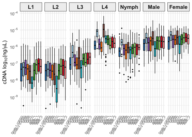
Boxplot interstades
# 1) Ensure factor orders
desired_order <- c(
  "Dnab-1 (GP02)", "Dnab-2 (GP02)", "GP05", "GP09",
  "GP11", "GP12", "RelB_1", "RelE_1", "RelB_2", "RelE_2"
)
stage_order <- c("L1", "L2", "L3", "L4", "Nymph", "Male", "Female")

data_combined$GENE  <- factor(data_combined$GENE,  levels = desired_order)
data_combined$Stage <- factor(data_combined$Stage, levels = stage_order)

# 2) Custom color palette (paired hues for linked genes)
gene_colors <- c(
  # GP02 pair: blue (dark/light)
  "Dnab-1 (GP02)" = "#2C7FB8",  # dark/medium blue
  "Dnab-2 (GP02)" = "#A6CEE3",  # light blue

  # Distinct colors for the other GPs
  "GP05"          = "#9467BD",  # purple
  "GP09"          = "#FF7F00",  # orange
  "GP11"          = "#8C564B",  # brown
  "GP12"          = "#17BECF",  # teal

  # Rel_1 pair: green (dark/light)
  "RelB_1"        = "#33A02C",  # dark/medium green
  "RelE_1"        = "#B2DF8A",  # light green

  # Rel_2 pair: red (dark/light) — now same-hue gradient
  "RelB_2"        = "#E31A1C",  # strong red
  "RelE_2"        = "#FCA5A5"   # light red (slightly lighter than FB9A99)
)

library(ggplot2)
library(dplyr)

ggplot(
  data_combined %>% dplyr::filter(GENE != "wsp"),
  aes(x = GENE, y = concentration, fill = GENE)
) +
  geom_boxplot(outlier.size = 0.8, width = 0.7, color = "black") +
  facet_wrap(~Stage, nrow = 1) +
  scale_y_log10(
    labels = scales::label_log(),
    breaks = scales::trans_breaks("log10", function(x) 10^x)
  ) +
  labs(
    y = expression("cDNA " * log[10] * "(ng/" * mu * "L)"),
    x = NULL
  ) +
  scale_fill_manual(values = gene_colors, breaks = desired_order) +
  theme_minimal(base_size = 13) +
  theme(
    axis.text.x = element_text(angle = 60, hjust = 1, size = 8),
    strip.text = element_text(size = 14, face = "bold"),
    axis.title = element_text(size = 14),
    axis.text = element_text(size = 11),
    legend.position = "none",
    strip.background = element_rect(fill = "#f0f0f0", color = "black")
  )
ggsave(
  filename = "./Figures/Sup_5/Boxplots_interstage.svg",
  width = 10,
  height = 5,
  units = "in"
)
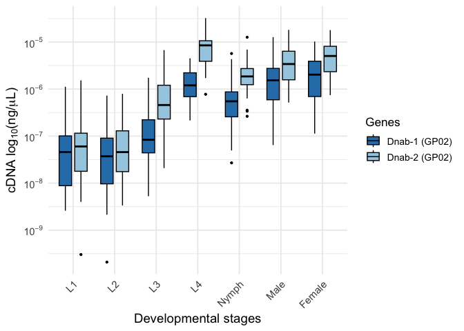
Boxplot inter-stages zoom on Dnab-1 and Dnab-2
library(dplyr)
library(ggplot2)

# enforce the Stage order
stage_order <- c("L1", "L2", "L3", "L4", "Nymph", "Male", "Female")

p <- ggplot(
  data_combined %>%
    filter(GENE %in% c("Dnab-1 (GP02)", "Dnab-2 (GP02)")) %>%
    mutate(
      GENE  = factor(GENE, levels = c("Dnab-1 (GP02)", "Dnab-2 (GP02)")),
      Stage = factor(Stage, levels = stage_order)
    ),
  aes(x = Stage, y = concentration, fill = GENE)
) +
  geom_boxplot(
    position = position_dodge(width = 0.75),
    outlier.size = 0.8,
    width = 0.6,
    color = "black"
  ) +
  scale_y_log10(
    labels = scales::label_log(),
    breaks = scales::trans_breaks("log10", function(x) 10^x)
  ) +
  labs(
    y = expression("cDNA " * log[10] * "(ng/" * mu * "L)"),
    x = "Developmental stages",
    fill = "Genes"
  ) +
  # 🔵 Custom colors for the GP02 pair
  scale_fill_manual(
    values = c(
      "Dnab-1 (GP02)" = "#2C7FB8",  # dark/medium blue
      "Dnab-2 (GP02)" = "#A6CEE3"   # light blue
    ),
    breaks = c("Dnab-1 (GP02)", "Dnab-2 (GP02)")  # keep legend order consistent
  ) +
  theme_minimal(base_size = 13) +
  theme(
    axis.text.x = element_text(angle = 45, hjust = 1),
    axis.title  = element_text(size = 14),
    axis.text   = element_text(size = 11)
  )

p
ggsave(
  filename = "./Figures/Sup_5/Dnab1_Dnab2_expression_by_stage.svg",
  plot = p,
  width = 10,
  height = 5,
  units = "in"
)