RosaBioinfo
Intra-stage statistics of expression of pWCP genes in Wolbachia endosymbiont of Culex using RT-qPCR concentrations
Mateo Jarry
2026-01-22
Data loading
This notebook needs in input “Data/Culex_SLAB_design.xlsx” (get here).
library(readxl)
library(ggplot2)
library(dplyr)
##
## Attaching package: 'dplyr'

## The following objects are masked from 'package:stats':
##
##     filter, lag

## The following objects are masked from 'package:base':
##
##     intersect, setdiff, setequal, union
library(glmmTMB)
## Warning in checkDepPackageVersion(dep_pkg = "TMB"): Package version inconsistency detected.
## glmmTMB was built with TMB version 1.9.10
## Current TMB version is 1.9.11
## Please re-install glmmTMB from source or restore original 'TMB' package (see '?reinstalling' for more information)
library(emmeans)
## Warning: package 'emmeans' was built under R version 4.3.3

## Welcome to emmeans.
## Caution: You lose important information if you filter this package's results.
## See '? untidy'
library(stringr)
library(purrr)
library(openxlsx)
## Warning: package 'openxlsx' was built under R version 4.3.3
library(tibble)
data <- read_excel('./Data/Culex_SLAB_design.xlsx', sheet = 'R_data_expression')
str(data)
## tibble [2,310 × 5] (S3: tbl_df/tbl/data.frame)
##  $ ID_tube           : chr [1:2310] "SLAB_F_1" "SLAB_F_2" "SLAB_F_3" "SLAB_F_4" ...
##  $ Stage             : chr [1:2310] "Female" "Female" "Female" "Female" ...
##  $ Plate             : chr [1:2310] "qPCR_MJ1" "qPCR_MJ1" "qPCR_MJ1" "qPCR_MJ1" ...
##  $ GENE              : chr [1:2310] "wsp" "wsp" "wsp" "wsp" ...
##  $ Concentration Mean: chr [1:2310] "9.7399999999999999E-8" "1.801E-7" "1.4999999999999999E-7" "4.2E-7" ...
data$GENE <- as.factor(data$GENE)
data$Plate <- as.factor(data$Plate)
data$Stage <- as.factor(data$Stage)
data$concentration <- as.numeric(data$`Concentration Mean`)
## Warning: NAs introduced by coercion
data_cleaned <- na.omit(data)
data_cleaned <- data.frame(data_cleaned)
summary(data_cleaned)
##    ID_tube             Stage           Plate                 GENE
##  Length:2258        Female:330   qPCR_MJ1 :  88   Dnab-1 (GP02): 207
##  Class :character   L1    :287   qPCR_MJ10:  88   RelB_1       : 207
##  Mode  :character   L2    :322   qPCR_MJ11:  88   RelE_2       : 207
##                     L3    :329   qPCR_MJ12:  88   Dnab-2 (GP02): 206
##                     L4    :330   qPCR_MJ14:  88   GP09         : 206
##                     Male  :330   qPCR_MJ15:  88   RelB_2       : 206
##                     Nymph :330   (Other)  :1730   (Other)      :1019
##  Concentration.Mean concentration
##  Length:2258        Min.   :2.100e-10
##  Class :character   1st Qu.:7.464e-08
##  Mode  :character   Median :5.360e-07
##                     Mean   :2.459e-06
##                     3rd Qu.:2.105e-06
##                     Max.   :1.750e-04
##
Data sorting and cleaning
library(dplyr)

# Filter dataset for Male stage
data_male <- data_cleaned %>% filter(Stage == "Male")

data_female <- data_cleaned %>% filter(Stage == "Female")

# Deletion of a female F12 (anormaly high cDNA concentration)
data_withoutF12 <- data_female %>% filter(ID_tube != "SLAB_F_12")

data_nymph <- data_cleaned %>% filter(Stage == "Nymph")

data_L4 <- data_cleaned %>% filter(Stage == "L4")

# Deletion of a female L4_24 (anormaly high cDNA concentration)

data_withoutL4_24 <- data_L4 %>% filter(ID_tube != "SLAB_L4_24")

data_L3 <- data_cleaned %>% filter(Stage == "L3")

data_L2 <- data_cleaned %>% filter(Stage == "L2")

data_L1 <- data_cleaned %>% filter(Stage == "L1")

# Add a 'Stage' column to each dataset
data_male$Stage <- "Male"
data_female$Stage <- "Female"
data_nymph$Stage <- "Nymph"
data_L4$Stage <- "L4"
data_L3$Stage <- "L3"
data_L2$Stage <- "L2"
data_L1$Stage <- "L1"

# Fuse the datasets
data_combined <- bind_rows(data_L1, data_L2, data_L3, data_withoutL4_24, data_nymph, data_male, data_withoutF12)
Intrastage analyses
Female stage
GLM with Gamma distribution and random variable for qPCR plates for SLAB mosquitoes
library(glmmTMB)

# Adjust Gamma GLMM model with random effect for "qPCR plates"
model_glmm <- glmmTMB(concentration ~ GENE + (1 | Plate),
                      data = data_withoutF12,
                      family = Gamma(link = "log"))

# Model summary
summary(model_glmm)
##  Family: Gamma  ( log )
## Formula:          concentration ~ GENE + (1 | Plate)
## Data: data_withoutF12
##
##      AIC      BIC   logLik deviance df.resid
##    -7418    -7369     3722    -7444      306
##
## Random effects:
##
## Conditional model:
##  Groups Name        Variance Std.Dev.
##  Plate  (Intercept) 0.2528   0.5028
## Number of obs: 319, groups:  Plate, 4
##
## Dispersion estimate for Gamma family (sigma^2): 0.619
##
## Conditional model:
##                   Estimate Std. Error z value Pr(>|z|)
## (Intercept)       -12.9360     0.2909  -44.47  < 2e-16 ***
## GENEDnab-2 (GP02)   0.7893     0.2068    3.82 0.000135 ***
## GENEGP05            0.2579     0.2068    1.25 0.212350
## GENEGP09            0.3490     0.2068    1.69 0.091421 .
## GENEGP11            0.6468     0.2069    3.13 0.001772 **
## GENEGP12           -0.1962     0.2077   -0.94 0.344917
## GENERelB_1          0.3878     0.2068    1.88 0.060753 .
## GENERelB_2          0.6445     0.2069    3.11 0.001842 **
## GENERelE_1          0.6432     0.2074    3.10 0.001927 **
## GENERelE_2          0.4689     0.2069    2.27 0.023455 *
## GENEwsp            -0.7242     0.2068   -3.50 0.000460 ***
## ---
## Signif. codes:  0 '***' 0.001 '**' 0.01 '*' 0.05 '.' 0.1 ' ' 1
# Post-hoc comparisons between genes
emm_glmm <- emmeans(model_glmm, ~ GENE)
post_hoc_glmm <- pairs(emm_glmm, adjust = "bonferroni")
print(post_hoc_glmm)
##  contrast                          estimate    SE  df z.ratio p.value
##  (Dnab-1 (GP02)) - (Dnab-2 (GP02)) -0.78935 0.207 Inf  -3.817  0.0074
##  (Dnab-1 (GP02)) - GP05            -0.25788 0.207 Inf  -1.247  1.0000
##  (Dnab-1 (GP02)) - GP09            -0.34899 0.207 Inf  -1.688  1.0000
##  (Dnab-1 (GP02)) - GP11            -0.64684 0.207 Inf  -3.126  0.0975
##  (Dnab-1 (GP02)) - GP12             0.19619 0.208 Inf   0.944  1.0000
##  (Dnab-1 (GP02)) - RelB_1          -0.38781 0.207 Inf  -1.875  1.0000
##  (Dnab-1 (GP02)) - RelB_2          -0.64447 0.207 Inf  -3.115  0.1013
##  (Dnab-1 (GP02)) - RelE_1          -0.64316 0.207 Inf  -3.101  0.1060
##  (Dnab-1 (GP02)) - RelE_2          -0.46891 0.207 Inf  -2.266  1.0000
##  (Dnab-1 (GP02)) - wsp              0.72420 0.207 Inf   3.503  0.0253
##  (Dnab-2 (GP02)) - GP05             0.53147 0.207 Inf   2.572  0.5568
##  (Dnab-2 (GP02)) - GP09             0.44036 0.207 Inf   2.130  1.0000
##  (Dnab-2 (GP02)) - GP11             0.14251 0.207 Inf   0.690  1.0000
##  (Dnab-2 (GP02)) - GP12             0.98554 0.208 Inf   4.734  0.0001
##  (Dnab-2 (GP02)) - RelB_1           0.40154 0.207 Inf   1.943  1.0000
##  (Dnab-2 (GP02)) - RelB_2           0.14488 0.207 Inf   0.700  1.0000
##  (Dnab-2 (GP02)) - RelE_1           0.14618 0.207 Inf   0.707  1.0000
##  (Dnab-2 (GP02)) - RelE_2           0.32043 0.207 Inf   1.550  1.0000
##  (Dnab-2 (GP02)) - wsp              1.51354 0.207 Inf   7.321  <.0001
##  GP05 - GP09                       -0.09111 0.207 Inf  -0.441  1.0000
##  GP05 - GP11                       -0.38896 0.207 Inf  -1.882  1.0000
##  GP05 - GP12                        0.45407 0.208 Inf   2.185  1.0000
##  GP05 - RelB_1                     -0.12993 0.207 Inf  -0.629  1.0000
##  GP05 - RelB_2                     -0.38659 0.207 Inf  -1.867  1.0000
##  GP05 - RelE_1                     -0.38528 0.207 Inf  -1.862  1.0000
##  GP05 - RelE_2                     -0.21103 0.207 Inf  -1.020  1.0000
##  GP05 - wsp                         0.98208 0.207 Inf   4.752  0.0001
##  GP09 - GP11                       -0.29785 0.207 Inf  -1.441  1.0000
##  GP09 - GP12                        0.54518 0.208 Inf   2.620  0.4830
##  GP09 - RelB_1                     -0.03882 0.207 Inf  -0.188  1.0000
##  GP09 - RelB_2                     -0.29548 0.207 Inf  -1.428  1.0000
##  GP09 - RelE_1                     -0.29417 0.207 Inf  -1.421  1.0000
##  GP09 - RelE_2                     -0.11992 0.207 Inf  -0.580  1.0000
##  GP09 - wsp                         1.07319 0.207 Inf   5.191  <.0001
##  GP11 - GP12                        0.84303 0.208 Inf   4.052  0.0028
##  GP11 - RelB_1                      0.25903 0.207 Inf   1.253  1.0000
##  GP11 - RelB_2                      0.00237 0.207 Inf   0.011  1.0000
##  GP11 - RelE_1                      0.00368 0.207 Inf   0.018  1.0000
##  GP11 - RelE_2                      0.17793 0.207 Inf   0.860  1.0000
##  GP11 - wsp                         1.37103 0.207 Inf   6.632  <.0001
##  GP12 - RelB_1                     -0.58400 0.208 Inf  -2.808  0.2744
##  GP12 - RelB_2                     -0.84066 0.209 Inf  -4.023  0.0032
##  GP12 - RelE_1                     -0.83935 0.209 Inf  -4.021  0.0032
##  GP12 - RelE_2                     -0.66510 0.209 Inf  -3.185  0.0796
##  GP12 - wsp                         0.52800 0.208 Inf   2.544  0.6020
##  RelB_1 - RelB_2                   -0.25666 0.207 Inf  -1.240  1.0000
##  RelB_1 - RelE_1                   -0.25536 0.207 Inf  -1.234  1.0000
##  RelB_1 - RelE_2                   -0.08111 0.207 Inf  -0.392  1.0000
##  RelB_1 - wsp                       1.11200 0.207 Inf   5.380  <.0001
##  RelB_2 - RelE_1                    0.00131 0.207 Inf   0.006  1.0000
##  RelB_2 - RelE_2                    0.17555 0.207 Inf   0.849  1.0000
##  RelB_2 - wsp                       1.36866 0.207 Inf   6.610  <.0001
##  RelE_1 - RelE_2                    0.17425 0.207 Inf   0.842  1.0000
##  RelE_1 - wsp                       1.36736 0.207 Inf   6.605  <.0001
##  RelE_2 - wsp                       1.19311 0.207 Inf   5.766  <.0001
##
## Results are given on the log (not the response) scale.
## P value adjustment: bonferroni method for 55 tests
Male stage
model_glmm <- glmmTMB(concentration ~ GENE + (1 | Plate),
                      data = data_male,
                      family = Gamma(link = "log"))

summary(model_glmm)
##  Family: Gamma  ( log )
## Formula:          concentration ~ GENE + (1 | Plate)
## Data: data_male
##
##      AIC      BIC   logLik deviance df.resid
##  -7903.8  -7854.4   3964.9  -7929.8      317
##
## Random effects:
##
## Conditional model:
##  Groups Name        Variance Std.Dev.
##  Plate  (Intercept) 0.7936   0.8908
## Number of obs: 330, groups:  Plate, 5
##
## Dispersion estimate for Gamma family (sigma^2): 0.729
##
## Conditional model:
##                   Estimate Std. Error z value Pr(>|z|)
## (Intercept)       -13.5171     0.4288 -31.523  < 2e-16 ***
## GENEDnab-2 (GP02)   0.9528     0.2211   4.309 1.64e-05 ***
## GENEGP05            0.1869     0.2206   0.847   0.3968
## GENEGP09            0.3250     0.2205   1.474   0.1405
## GENEGP11            0.8867     0.2209   4.013 5.99e-05 ***
## GENEGP12           -0.3935     0.2215  -1.777   0.0756 .
## GENERelB_1          0.3364     0.2205   1.525   0.1271
## GENERelB_2          0.4845     0.2213   2.189   0.0286 *
## GENERelE_1          0.5211     0.2207   2.361   0.0182 *
## GENERelE_2          0.4336     0.2209   1.963   0.0497 *
## GENEwsp            -0.3898     0.2212  -1.763   0.0779 .
## ---
## Signif. codes:  0 '***' 0.001 '**' 0.01 '*' 0.05 '.' 0.1 ' ' 1
emm_glmm <- emmeans(model_glmm, ~ GENE)
post_hoc_glmm <- pairs(emm_glmm, adjust = "bonferroni")
print(post_hoc_glmm)
##  contrast                          estimate    SE  df z.ratio p.value
##  (Dnab-1 (GP02)) - (Dnab-2 (GP02)) -0.95276 0.221 Inf  -4.309  0.0009
##  (Dnab-1 (GP02)) - GP05            -0.18692 0.221 Inf  -0.847  1.0000
##  (Dnab-1 (GP02)) - GP09            -0.32502 0.221 Inf  -1.474  1.0000
##  (Dnab-1 (GP02)) - GP11            -0.88666 0.221 Inf  -4.013  0.0033
##  (Dnab-1 (GP02)) - GP12             0.39346 0.221 Inf   1.777  1.0000
##  (Dnab-1 (GP02)) - RelB_1          -0.33639 0.221 Inf  -1.525  1.0000
##  (Dnab-1 (GP02)) - RelB_2          -0.48455 0.221 Inf  -2.189  1.0000
##  (Dnab-1 (GP02)) - RelE_1          -0.52109 0.221 Inf  -2.361  1.0000
##  (Dnab-1 (GP02)) - RelE_2          -0.43358 0.221 Inf  -1.963  1.0000
##  (Dnab-1 (GP02)) - wsp              0.38985 0.221 Inf   1.763  1.0000
##  (Dnab-2 (GP02)) - GP05             0.76584 0.221 Inf   3.471  0.0285
##  (Dnab-2 (GP02)) - GP09             0.62773 0.221 Inf   2.844  0.2454
##  (Dnab-2 (GP02)) - GP11             0.06610 0.223 Inf   0.297  1.0000
##  (Dnab-2 (GP02)) - GP12             1.34621 0.223 Inf   6.027  <.0001
##  (Dnab-2 (GP02)) - RelB_1           0.61637 0.221 Inf   2.789  0.2903
##  (Dnab-2 (GP02)) - RelB_2           0.46821 0.221 Inf   2.122  1.0000
##  (Dnab-2 (GP02)) - RelE_1           0.43167 0.221 Inf   1.954  1.0000
##  (Dnab-2 (GP02)) - RelE_2           0.51918 0.221 Inf   2.349  1.0000
##  (Dnab-2 (GP02)) - wsp              1.34261 0.223 Inf   6.031  <.0001
##  GP05 - GP09                       -0.13810 0.220 Inf  -0.626  1.0000
##  GP05 - GP11                       -0.69974 0.222 Inf  -3.157  0.0877
##  GP05 - GP12                        0.58038 0.222 Inf   2.611  0.4970
##  GP05 - RelB_1                     -0.14947 0.221 Inf  -0.678  1.0000
##  GP05 - RelB_2                     -0.29763 0.221 Inf  -1.348  1.0000
##  GP05 - RelE_1                     -0.33417 0.221 Inf  -1.514  1.0000
##  GP05 - RelE_2                     -0.24666 0.221 Inf  -1.117  1.0000
##  GP05 - wsp                         0.57677 0.222 Inf   2.602  0.5101
##  GP09 - GP11                       -0.56164 0.221 Inf  -2.537  0.6151
##  GP09 - GP12                        0.71848 0.222 Inf   3.239  0.0661
##  GP09 - RelB_1                     -0.01136 0.220 Inf  -0.052  1.0000
##  GP09 - RelB_2                     -0.15952 0.221 Inf  -0.722  1.0000
##  GP09 - RelE_1                     -0.19607 0.221 Inf  -0.888  1.0000
##  GP09 - RelE_2                     -0.10855 0.221 Inf  -0.492  1.0000
##  GP09 - wsp                         0.71487 0.222 Inf   3.225  0.0692
##  GP11 - GP12                        1.28012 0.221 Inf   5.801  <.0001
##  GP11 - RelB_1                      0.55027 0.221 Inf   2.488  0.7060
##  GP11 - RelB_2                      0.40211 0.223 Inf   1.802  1.0000
##  GP11 - RelE_1                      0.36557 0.222 Inf   1.650  1.0000
##  GP11 - RelE_2                      0.45308 0.222 Inf   2.042  1.0000
##  GP11 - wsp                         1.27651 0.221 Inf   5.771  <.0001
##  GP12 - RelB_1                     -0.72984 0.221 Inf  -3.295  0.0541
##  GP12 - RelB_2                     -0.87800 0.224 Inf  -3.917  0.0049
##  GP12 - RelE_1                     -0.91455 0.223 Inf  -4.110  0.0022
##  GP12 - RelE_2                     -0.82703 0.223 Inf  -3.717  0.0111
##  GP12 - wsp                        -0.00361 0.222 Inf  -0.016  1.0000
##  RelB_1 - RelB_2                   -0.14816 0.221 Inf  -0.669  1.0000
##  RelB_1 - RelE_1                   -0.18470 0.221 Inf  -0.836  1.0000
##  RelB_1 - RelE_2                   -0.09719 0.221 Inf  -0.440  1.0000
##  RelB_1 - wsp                       0.72623 0.222 Inf   3.277  0.0577
##  RelB_2 - RelE_1                   -0.03654 0.221 Inf  -0.165  1.0000
##  RelB_2 - RelE_2                    0.05097 0.221 Inf   0.230  1.0000
##  RelB_2 - wsp                       0.87440 0.222 Inf   3.932  0.0046
##  RelE_1 - RelE_2                    0.08751 0.221 Inf   0.397  1.0000
##  RelE_1 - wsp                       0.91094 0.221 Inf   4.121  0.0021
##  RelE_2 - wsp                       0.82343 0.221 Inf   3.719  0.0110
##
## Results are given on the log (not the response) scale.
## P value adjustment: bonferroni method for 55 tests
Nymph stage
model_glmm <- glmmTMB(concentration ~ GENE + (1 | Plate),
                      data = data_nymph,
                      family = Gamma(link = "log"))

summary(model_glmm)
##  Family: Gamma  ( log )
## Formula:          concentration ~ GENE + (1 | Plate)
## Data: data_nymph
##
##      AIC      BIC   logLik deviance df.resid
##  -8464.3  -8414.9   4245.1  -8490.3      317
##
## Random effects:
##
## Conditional model:
##  Groups Name        Variance Std.Dev.
##  Plate  (Intercept) 0.2793   0.5285
## Number of obs: 330, groups:  Plate, 5
##
## Dispersion estimate for Gamma family (sigma^2): 0.778
##
## Conditional model:
##                   Estimate Std. Error z value Pr(>|z|)
## (Intercept)       -14.2082     0.2878  -49.36  < 2e-16 ***
## GENEDnab-2 (GP02)   1.4109     0.2299    6.14 8.45e-10 ***
## GENEGP05            0.3249     0.2279    1.43   0.1539
## GENEGP09            0.1930     0.2280    0.85   0.3974
## GENEGP11            0.4518     0.2295    1.97   0.0490 *
## GENEGP12            0.2032     0.2289    0.89   0.3746
## GENERelB_1          0.4046     0.2281    1.77   0.0762 .
## GENERelB_2          0.5503     0.2282    2.41   0.0159 *
## GENERelE_1          0.4832     0.2283    2.12   0.0343 *
## GENERelE_2          0.4741     0.2285    2.07   0.0380 *
## GENEwsp            -0.5796     0.2283   -2.54   0.0111 *
## ---
## Signif. codes:  0 '***' 0.001 '**' 0.01 '*' 0.05 '.' 0.1 ' ' 1
emm_glmm <- emmeans(model_glmm, ~ GENE)
post_hoc_glmm <- pairs(emm_glmm, adjust = "bonferroni")
print(post_hoc_glmm)
##  contrast                          estimate    SE  df z.ratio p.value
##  (Dnab-1 (GP02)) - (Dnab-2 (GP02)) -1.41092 0.230 Inf  -6.136  <.0001
##  (Dnab-1 (GP02)) - GP05            -0.32490 0.228 Inf  -1.426  1.0000
##  (Dnab-1 (GP02)) - GP09            -0.19297 0.228 Inf  -0.846  1.0000
##  (Dnab-1 (GP02)) - GP11            -0.45183 0.230 Inf  -1.969  1.0000
##  (Dnab-1 (GP02)) - GP12            -0.20324 0.229 Inf  -0.888  1.0000
##  (Dnab-1 (GP02)) - RelB_1          -0.40457 0.228 Inf  -1.773  1.0000
##  (Dnab-1 (GP02)) - RelB_2          -0.55025 0.228 Inf  -2.412  0.8736
##  (Dnab-1 (GP02)) - RelE_1          -0.48323 0.228 Inf  -2.117  1.0000
##  (Dnab-1 (GP02)) - RelE_2          -0.47406 0.228 Inf  -2.075  1.0000
##  (Dnab-1 (GP02)) - wsp              0.57961 0.228 Inf   2.538  0.6124
##  (Dnab-2 (GP02)) - GP05             1.08602 0.230 Inf   4.725  0.0001
##  (Dnab-2 (GP02)) - GP09             1.21795 0.230 Inf   5.286  <.0001
##  (Dnab-2 (GP02)) - GP11             0.95909 0.232 Inf   4.132  0.0020
##  (Dnab-2 (GP02)) - GP12             1.20768 0.231 Inf   5.222  <.0001
##  (Dnab-2 (GP02)) - RelB_1           1.00635 0.231 Inf   4.364  0.0007
##  (Dnab-2 (GP02)) - RelB_2           0.86067 0.229 Inf   3.762  0.0093
##  (Dnab-2 (GP02)) - RelE_1           0.92769 0.229 Inf   4.051  0.0028
##  (Dnab-2 (GP02)) - RelE_2           0.93686 0.230 Inf   4.076  0.0025
##  (Dnab-2 (GP02)) - wsp              1.99053 0.230 Inf   8.662  <.0001
##  GP05 - GP09                        0.13193 0.228 Inf   0.579  1.0000
##  GP05 - GP11                       -0.12693 0.229 Inf  -0.554  1.0000
##  GP05 - GP12                        0.12166 0.229 Inf   0.530  1.0000
##  GP05 - RelB_1                     -0.07967 0.228 Inf  -0.350  1.0000
##  GP05 - RelB_2                     -0.22535 0.228 Inf  -0.988  1.0000
##  GP05 - RelE_1                     -0.15833 0.228 Inf  -0.694  1.0000
##  GP05 - RelE_2                     -0.14916 0.228 Inf  -0.654  1.0000
##  GP05 - wsp                         0.90451 0.228 Inf   3.967  0.0040
##  GP09 - GP11                       -0.25886 0.228 Inf  -1.133  1.0000
##  GP09 - GP12                       -0.01027 0.230 Inf  -0.045  1.0000
##  GP09 - RelB_1                     -0.21160 0.228 Inf  -0.928  1.0000
##  GP09 - RelB_2                     -0.35728 0.228 Inf  -1.565  1.0000
##  GP09 - RelE_1                     -0.29026 0.228 Inf  -1.272  1.0000
##  GP09 - RelE_2                     -0.28109 0.228 Inf  -1.233  1.0000
##  GP09 - wsp                         0.77258 0.228 Inf   3.387  0.0388
##  GP11 - GP12                        0.24859 0.233 Inf   1.066  1.0000
##  GP11 - RelB_1                      0.04726 0.229 Inf   0.207  1.0000
##  GP11 - RelB_2                     -0.09842 0.229 Inf  -0.429  1.0000
##  GP11 - RelE_1                     -0.03140 0.229 Inf  -0.137  1.0000
##  GP11 - RelE_2                     -0.02223 0.228 Inf  -0.097  1.0000
##  GP11 - wsp                         1.03144 0.229 Inf   4.512  0.0004
##  GP12 - RelB_1                     -0.20133 0.230 Inf  -0.874  1.0000
##  GP12 - RelB_2                     -0.34701 0.230 Inf  -1.509  1.0000
##  GP12 - RelE_1                     -0.27999 0.230 Inf  -1.217  1.0000
##  GP12 - RelE_2                     -0.27082 0.231 Inf  -1.171  1.0000
##  GP12 - wsp                         0.78285 0.231 Inf   3.392  0.0382
##  RelB_1 - RelB_2                   -0.14568 0.228 Inf  -0.638  1.0000
##  RelB_1 - RelE_1                   -0.07866 0.228 Inf  -0.344  1.0000
##  RelB_1 - RelE_2                   -0.06949 0.228 Inf  -0.305  1.0000
##  RelB_1 - wsp                       0.98418 0.228 Inf   4.318  0.0009
##  RelB_2 - RelE_1                    0.06702 0.228 Inf   0.294  1.0000
##  RelB_2 - RelE_2                    0.07619 0.228 Inf   0.334  1.0000
##  RelB_2 - wsp                       1.12986 0.228 Inf   4.954  <.0001
##  RelE_1 - RelE_2                    0.00917 0.228 Inf   0.040  1.0000
##  RelE_1 - wsp                       1.06284 0.228 Inf   4.655  0.0002
##  RelE_2 - wsp                       1.05367 0.228 Inf   4.623  0.0002
##
## Results are given on the log (not the response) scale.
## P value adjustment: bonferroni method for 55 tests
L4 stage
model_glmm <- glmmTMB(concentration ~ GENE + (1 | Plate),
                      data = data_L4,
                      family = Gamma(link = "log"))

summary(model_glmm)
##  Family: Gamma  ( log )
## Formula:          concentration ~ GENE + (1 | Plate)
## Data: data_L4
##
##      AIC      BIC   logLik deviance df.resid
##  -7970.4  -7921.0   3998.2  -7996.4      317
##
## Random effects:
##
## Conditional model:
##  Groups Name        Variance Std.Dev.
##  Plate  (Intercept) 0.6359   0.7974
## Number of obs: 330, groups:  Plate, 4
##
## Dispersion estimate for Gamma family (sigma^2): 0.397
##
## Conditional model:
##                    Estimate Std. Error z value Pr(>|z|)
## (Intercept)       -13.61344    0.41509  -32.80  < 2e-16 ***
## GENEDnab-2 (GP02)   1.90093    0.16308   11.66  < 2e-16 ***
## GENEGP05            0.24123    0.16294    1.48  0.13876
## GENEGP09           -0.09316    0.16308   -0.57  0.56781
## GENEGP11            2.30893    0.16590   13.92  < 2e-16 ***
## GENEGP12            0.66605    0.16316    4.08 4.46e-05 ***
## GENERelB_1          0.74412    0.16274    4.57 4.82e-06 ***
## GENERelB_2          0.50282    0.16287    3.09  0.00202 **
## GENERelE_1          0.31650    0.16318    1.94  0.05243 .
## GENERelE_2          0.34220    0.16286    2.10  0.03563 *
## GENEwsp            -0.64509    0.16282   -3.96 7.43e-05 ***
## ---
## Signif. codes:  0 '***' 0.001 '**' 0.01 '*' 0.05 '.' 0.1 ' ' 1
emm_glmm <- emmeans(model_glmm, ~ GENE)
post_hoc_glmm <- pairs(emm_glmm, adjust = "bonferroni")
print(post_hoc_glmm)
##  contrast                          estimate    SE  df z.ratio p.value
##  (Dnab-1 (GP02)) - (Dnab-2 (GP02))  -1.9009 0.163 Inf -11.657  <.0001
##  (Dnab-1 (GP02)) - GP05             -0.2412 0.163 Inf  -1.480  1.0000
##  (Dnab-1 (GP02)) - GP09              0.0932 0.163 Inf   0.571  1.0000
##  (Dnab-1 (GP02)) - GP11             -2.3089 0.166 Inf -13.918  <.0001
##  (Dnab-1 (GP02)) - GP12             -0.6661 0.163 Inf  -4.082  0.0025
##  (Dnab-1 (GP02)) - RelB_1           -0.7441 0.163 Inf  -4.573  0.0003
##  (Dnab-1 (GP02)) - RelB_2           -0.5028 0.163 Inf  -3.087  0.1111
##  (Dnab-1 (GP02)) - RelE_1           -0.3165 0.163 Inf  -1.940  1.0000
##  (Dnab-1 (GP02)) - RelE_2           -0.3422 0.163 Inf  -2.101  1.0000
##  (Dnab-1 (GP02)) - wsp               0.6451 0.163 Inf   3.962  0.0041
##  (Dnab-2 (GP02)) - GP05              1.6597 0.163 Inf  10.193  <.0001
##  (Dnab-2 (GP02)) - GP09              1.9941 0.163 Inf  12.241  <.0001
##  (Dnab-2 (GP02)) - GP11             -0.4080 0.166 Inf  -2.452  0.7821
##  (Dnab-2 (GP02)) - GP12              1.2349 0.164 Inf   7.526  <.0001
##  (Dnab-2 (GP02)) - RelB_1            1.1568 0.163 Inf   7.092  <.0001
##  (Dnab-2 (GP02)) - RelB_2            1.3981 0.163 Inf   8.577  <.0001
##  (Dnab-2 (GP02)) - RelE_1            1.5844 0.163 Inf   9.728  <.0001
##  (Dnab-2 (GP02)) - RelE_2            1.5587 0.163 Inf   9.567  <.0001
##  (Dnab-2 (GP02)) - wsp               2.5460 0.163 Inf  15.614  <.0001
##  GP05 - GP09                         0.3344 0.163 Inf   2.053  1.0000
##  GP05 - GP11                        -2.0677 0.166 Inf -12.489  <.0001
##  GP05 - GP12                        -0.4248 0.164 Inf  -2.595  0.5204
##  GP05 - RelB_1                      -0.5029 0.163 Inf  -3.086  0.1115
##  GP05 - RelB_2                      -0.2616 0.163 Inf  -1.607  1.0000
##  GP05 - RelE_1                      -0.0753 0.163 Inf  -0.462  1.0000
##  GP05 - RelE_2                      -0.1010 0.163 Inf  -0.620  1.0000
##  GP05 - wsp                          0.8863 0.163 Inf   5.443  <.0001
##  GP09 - GP11                        -2.4021 0.165 Inf -14.553  <.0001
##  GP09 - GP12                        -0.7592 0.164 Inf  -4.641  0.0002
##  GP09 - RelB_1                      -0.8373 0.163 Inf  -5.137  <.0001
##  GP09 - RelB_2                      -0.5960 0.163 Inf  -3.658  0.0140
##  GP09 - RelE_1                      -0.4097 0.163 Inf  -2.511  0.6614
##  GP09 - RelE_2                      -0.4354 0.163 Inf  -2.672  0.4145
##  GP09 - wsp                          0.5519 0.163 Inf   3.388  0.0387
##  GP11 - GP12                         1.6429 0.165 Inf   9.962  <.0001
##  GP11 - RelB_1                       1.5648 0.166 Inf   9.453  <.0001
##  GP11 - RelB_2                       1.8061 0.165 Inf  10.934  <.0001
##  GP11 - RelE_1                       1.9924 0.166 Inf  11.974  <.0001
##  GP11 - RelE_2                       1.9667 0.165 Inf  11.886  <.0001
##  GP11 - wsp                          2.9540 0.165 Inf  17.901  <.0001
##  GP12 - RelB_1                      -0.0781 0.163 Inf  -0.479  1.0000
##  GP12 - RelB_2                       0.1632 0.163 Inf   0.999  1.0000
##  GP12 - RelE_1                       0.3496 0.164 Inf   2.127  1.0000
##  GP12 - RelE_2                       0.3238 0.164 Inf   1.980  1.0000
##  GP12 - wsp                          1.3111 0.163 Inf   8.035  <.0001
##  RelB_1 - RelB_2                     0.2413 0.163 Inf   1.482  1.0000
##  RelB_1 - RelE_1                     0.4276 0.163 Inf   2.620  0.4843
##  RelB_1 - RelE_2                     0.4019 0.163 Inf   2.468  0.7479
##  RelB_1 - wsp                        1.3892 0.163 Inf   8.534  <.0001
##  RelB_2 - RelE_1                     0.1863 0.163 Inf   1.143  1.0000
##  RelB_2 - RelE_2                     0.1606 0.163 Inf   0.987  1.0000
##  RelB_2 - wsp                        1.1479 0.163 Inf   7.053  <.0001
##  RelE_1 - RelE_2                    -0.0257 0.163 Inf  -0.158  1.0000
##  RelE_1 - wsp                        0.9616 0.163 Inf   5.896  <.0001
##  RelE_2 - wsp                        0.9873 0.163 Inf   6.065  <.0001
##
## Results are given on the log (not the response) scale.
## P value adjustment: bonferroni method for 55 tests
L3 stage
model_glmm <- glmmTMB(concentration ~ GENE + (1 | Plate),
                      data = data_L3,
                      family = Gamma(link = "log"))

summary(model_glmm)
##  Family: Gamma  ( log )
## Formula:          concentration ~ GENE + (1 | Plate)
## Data: data_L3
##
##      AIC      BIC   logLik deviance df.resid
##  -9283.4  -9234.1   4654.7  -9309.4      316
##
## Random effects:
##
## Conditional model:
##  Groups Name        Variance Std.Dev.
##  Plate  (Intercept) 0.4671   0.6834
## Number of obs: 329, groups:  Plate, 4
##
## Dispersion estimate for Gamma family (sigma^2): 1.26
##
## Conditional model:
##                   Estimate Std. Error z value Pr(>|z|)
## (Intercept)       -15.6036     0.3989  -39.11  < 2e-16 ***
## GENEDnab-2 (GP02)   1.6813     0.2957    5.69 1.31e-08 ***
## GENEGP05            0.3761     0.2902    1.30  0.19491
## GENEGP09            0.1077     0.2907    0.37  0.71094
## GENEGP11            1.4753     0.3051    4.84 1.33e-06 ***
## GENEGP12           -0.6218     0.2940   -2.12  0.03439 *
## GENERelB_1          0.5738     0.2902    1.98  0.04805 *
## GENERelB_2          0.7972     0.2925    2.73  0.00643 **
## GENERelE_1          0.5058     0.2911    1.74  0.08227 .
## GENERelE_2          0.6373     0.2902    2.20  0.02808 *
## GENEwsp            -0.8507     0.2931   -2.90  0.00371 **
## ---
## Signif. codes:  0 '***' 0.001 '**' 0.01 '*' 0.05 '.' 0.1 ' ' 1
emm_glmm <- emmeans(model_glmm, ~ GENE)
post_hoc_glmm <- pairs(emm_glmm, adjust = "bonferroni")
print(post_hoc_glmm)
##  contrast                          estimate    SE  df z.ratio p.value
##  (Dnab-1 (GP02)) - (Dnab-2 (GP02))  -1.6813 0.296 Inf  -5.685  <.0001
##  (Dnab-1 (GP02)) - GP05             -0.3761 0.290 Inf  -1.296  1.0000
##  (Dnab-1 (GP02)) - GP09             -0.1077 0.291 Inf  -0.371  1.0000
##  (Dnab-1 (GP02)) - GP11             -1.4753 0.305 Inf  -4.835  0.0001
##  (Dnab-1 (GP02)) - GP12              0.6218 0.294 Inf   2.115  1.0000
##  (Dnab-1 (GP02)) - RelB_1           -0.5738 0.290 Inf  -1.977  1.0000
##  (Dnab-1 (GP02)) - RelB_2           -0.7972 0.293 Inf  -2.725  0.3536
##  (Dnab-1 (GP02)) - RelE_1           -0.5058 0.291 Inf  -1.738  1.0000
##  (Dnab-1 (GP02)) - RelE_2           -0.6373 0.290 Inf  -2.196  1.0000
##  (Dnab-1 (GP02)) - wsp               0.8507 0.293 Inf   2.902  0.2039
##  (Dnab-2 (GP02)) - GP05              1.3052 0.295 Inf   4.427  0.0005
##  (Dnab-2 (GP02)) - GP09              1.5736 0.299 Inf   5.257  <.0001
##  (Dnab-2 (GP02)) - GP11              0.2060 0.293 Inf   0.704  1.0000
##  (Dnab-2 (GP02)) - GP12              2.3032 0.291 Inf   7.911  <.0001
##  (Dnab-2 (GP02)) - RelB_1            1.1075 0.296 Inf   3.742  0.0100
##  (Dnab-2 (GP02)) - RelB_2            0.8841 0.302 Inf   2.929  0.1871
##  (Dnab-2 (GP02)) - RelE_1            1.1756 0.300 Inf   3.916  0.0049
##  (Dnab-2 (GP02)) - RelE_2            1.0440 0.294 Inf   3.545  0.0216
##  (Dnab-2 (GP02)) - wsp               2.5320 0.302 Inf   8.389  <.0001
##  GP05 - GP09                         0.2684 0.291 Inf   0.922  1.0000
##  GP05 - GP11                        -1.0992 0.304 Inf  -3.616  0.0164
##  GP05 - GP12                         0.9980 0.294 Inf   3.399  0.0373
##  GP05 - RelB_1                      -0.1977 0.290 Inf  -0.681  1.0000
##  GP05 - RelB_2                      -0.4210 0.293 Inf  -1.439  1.0000
##  GP05 - RelE_1                      -0.1296 0.291 Inf  -0.445  1.0000
##  GP05 - RelE_2                      -0.2611 0.290 Inf  -0.900  1.0000
##  GP05 - wsp                          1.2268 0.293 Inf   4.181  0.0016
##  GP09 - GP11                        -1.3676 0.310 Inf  -4.405  0.0006
##  GP09 - GP12                         0.7296 0.297 Inf   2.459  0.7661
##  GP09 - RelB_1                      -0.4661 0.291 Inf  -1.603  1.0000
##  GP09 - RelB_2                      -0.6895 0.291 Inf  -2.366  0.9887
##  GP09 - RelE_1                      -0.3980 0.290 Inf  -1.371  1.0000
##  GP09 - RelE_2                      -0.5296 0.291 Inf  -1.819  1.0000
##  GP09 - wsp                          0.9584 0.293 Inf   3.275  0.0581
##  GP11 - GP12                         2.0971 0.294 Inf   7.124  <.0001
##  GP11 - RelB_1                       0.9015 0.306 Inf   2.947  0.1767
##  GP11 - RelB_2                       0.6781 0.315 Inf   2.154  1.0000
##  GP11 - RelE_1                       0.9695 0.312 Inf   3.107  0.1038
##  GP11 - RelE_2                       0.8380 0.303 Inf   2.765  0.3135
##  GP11 - wsp                          2.3260 0.313 Inf   7.428  <.0001
##  GP12 - RelB_1                      -1.1956 0.295 Inf  -4.056  0.0027
##  GP12 - RelB_2                      -1.4190 0.300 Inf  -4.726  0.0001
##  GP12 - RelE_1                      -1.1276 0.298 Inf  -3.786  0.0084
##  GP12 - RelE_2                      -1.2591 0.293 Inf  -4.297  0.0010
##  GP12 - wsp                          0.2288 0.299 Inf   0.764  1.0000
##  RelB_1 - RelB_2                    -0.2234 0.292 Inf  -0.765  1.0000
##  RelB_1 - RelE_1                     0.0680 0.291 Inf   0.234  1.0000
##  RelB_1 - RelE_2                    -0.0635 0.290 Inf  -0.219  1.0000
##  RelB_1 - wsp                        1.4245 0.293 Inf   4.860  0.0001
##  RelB_2 - RelE_1                     0.2914 0.291 Inf   1.003  1.0000
##  RelB_2 - RelE_2                     0.1599 0.293 Inf   0.546  1.0000
##  RelB_2 - wsp                        1.6478 0.294 Inf   5.610  <.0001
##  RelE_1 - RelE_2                    -0.1315 0.292 Inf  -0.451  1.0000
##  RelE_1 - wsp                        1.3564 0.293 Inf   4.634  0.0002
##  RelE_2 - wsp                        1.4879 0.294 Inf   5.068  <.0001
##
## Results are given on the log (not the response) scale.
## P value adjustment: bonferroni method for 55 tests
L2 stage
model_glmm <- glmmTMB(concentration ~ GENE + (1 | Plate),
                      data = data_L2,
                      family = Gamma(link = "log"))

summary(model_glmm)
##  Family: Gamma  ( log )
## Formula:          concentration ~ GENE + (1 | Plate)
## Data: data_L2
##
##      AIC      BIC   logLik deviance df.resid
##   -10126   -10077     5076   -10152      309
##
## Random effects:
##
## Conditional model:
##  Groups Name        Variance Std.Dev.
##  Plate  (Intercept) 1.316    1.147
## Number of obs: 322, groups:  Plate, 5
##
## Dispersion estimate for Gamma family (sigma^2): 0.858
##
## Conditional model:
##                    Estimate Std. Error z value Pr(>|z|)
## (Intercept)       -17.06824    0.54177 -31.505  < 2e-16 ***
## GENEDnab-2 (GP02)   0.26641    0.23938   1.113  0.26574
## GENEGP05            0.16544    0.23923   0.692  0.48923
## GENEGP09            0.11945    0.23928   0.499  0.61764
## GENEGP11           -0.17373    0.24193  -0.718  0.47270
## GENEGP12           -1.44017    0.25829  -5.576 2.47e-08 ***
## GENERelB_1          0.02148    0.23941   0.090  0.92852
## GENERelB_2          0.61241    0.24013   2.550  0.01076 *
## GENERelE_1          0.66575    0.23961   2.778  0.00546 **
## GENERelE_2          0.44027    0.23930   1.840  0.06579 .
## GENEwsp            -1.31197    0.24137  -5.436 5.46e-08 ***
## ---
## Signif. codes:  0 '***' 0.001 '**' 0.01 '*' 0.05 '.' 0.1 ' ' 1
emm_glmm <- emmeans(model_glmm, ~ GENE)
post_hoc_glmm <- pairs(emm_glmm, adjust = "bonferroni")
print(post_hoc_glmm)
##  contrast                          estimate    SE  df z.ratio p.value
##  (Dnab-1 (GP02)) - (Dnab-2 (GP02))  -0.2664 0.239 Inf  -1.113  1.0000
##  (Dnab-1 (GP02)) - GP05             -0.1654 0.239 Inf  -0.692  1.0000
##  (Dnab-1 (GP02)) - GP09             -0.1194 0.239 Inf  -0.499  1.0000
##  (Dnab-1 (GP02)) - GP11              0.1737 0.242 Inf   0.718  1.0000
##  (Dnab-1 (GP02)) - GP12              1.4402 0.258 Inf   5.576  <.0001
##  (Dnab-1 (GP02)) - RelB_1           -0.0215 0.239 Inf  -0.090  1.0000
##  (Dnab-1 (GP02)) - RelB_2           -0.6124 0.240 Inf  -2.550  0.5920
##  (Dnab-1 (GP02)) - RelE_1           -0.6657 0.240 Inf  -2.778  0.3004
##  (Dnab-1 (GP02)) - RelE_2           -0.4403 0.239 Inf  -1.840  1.0000
##  (Dnab-1 (GP02)) - wsp               1.3120 0.241 Inf   5.436  <.0001
##  (Dnab-2 (GP02)) - GP05              0.1010 0.240 Inf   0.421  1.0000
##  (Dnab-2 (GP02)) - GP09              0.1470 0.240 Inf   0.613  1.0000
##  (Dnab-2 (GP02)) - GP11              0.4401 0.243 Inf   1.812  1.0000
##  (Dnab-2 (GP02)) - GP12              1.7066 0.257 Inf   6.638  <.0001
##  (Dnab-2 (GP02)) - RelB_1            0.2449 0.239 Inf   1.023  1.0000
##  (Dnab-2 (GP02)) - RelB_2           -0.3460 0.240 Inf  -1.442  1.0000
##  (Dnab-2 (GP02)) - RelE_1           -0.3993 0.239 Inf  -1.668  1.0000
##  (Dnab-2 (GP02)) - RelE_2           -0.1739 0.239 Inf  -0.727  1.0000
##  (Dnab-2 (GP02)) - wsp               1.5784 0.241 Inf   6.543  <.0001
##  GP05 - GP09                         0.0460 0.239 Inf   0.192  1.0000
##  GP05 - GP11                         0.3392 0.242 Inf   1.402  1.0000
##  GP05 - GP12                         1.6056 0.258 Inf   6.214  <.0001
##  GP05 - RelB_1                       0.1440 0.239 Inf   0.601  1.0000
##  GP05 - RelB_2                      -0.4470 0.240 Inf  -1.862  1.0000
##  GP05 - RelE_1                      -0.5003 0.239 Inf  -2.089  1.0000
##  GP05 - RelE_2                      -0.2748 0.239 Inf  -1.148  1.0000
##  GP05 - wsp                          1.4774 0.241 Inf   6.119  <.0001
##  GP09 - GP11                         0.2932 0.242 Inf   1.212  1.0000
##  GP09 - GP12                         1.5596 0.258 Inf   6.045  <.0001
##  GP09 - RelB_1                       0.0980 0.239 Inf   0.409  1.0000
##  GP09 - RelB_2                      -0.4930 0.240 Inf  -2.056  1.0000
##  GP09 - RelE_1                      -0.5463 0.239 Inf  -2.281  1.0000
##  GP09 - RelE_2                      -0.3208 0.239 Inf  -1.341  1.0000
##  GP09 - wsp                          1.4314 0.241 Inf   5.930  <.0001
##  GP11 - GP12                         1.2664 0.263 Inf   4.820  0.0001
##  GP11 - RelB_1                      -0.1952 0.242 Inf  -0.806  1.0000
##  GP11 - RelB_2                      -0.7861 0.243 Inf  -3.236  0.0667
##  GP11 - RelE_1                      -0.8395 0.243 Inf  -3.453  0.0305
##  GP11 - RelE_2                      -0.6140 0.243 Inf  -2.532  0.6246
##  GP11 - wsp                          1.1382 0.245 Inf   4.653  0.0002
##  GP12 - RelB_1                      -1.4616 0.258 Inf  -5.671  <.0001
##  GP12 - RelB_2                      -2.0526 0.259 Inf  -7.938  <.0001
##  GP12 - RelE_1                      -2.1059 0.257 Inf  -8.183  <.0001
##  GP12 - RelE_2                      -1.8804 0.257 Inf  -7.314  <.0001
##  GP12 - wsp                         -0.1282 0.259 Inf  -0.494  1.0000
##  RelB_1 - RelB_2                    -0.5909 0.239 Inf  -2.469  0.7462
##  RelB_1 - RelE_1                    -0.6443 0.239 Inf  -2.690  0.3925
##  RelB_1 - RelE_2                    -0.4188 0.239 Inf  -1.750  1.0000
##  RelB_1 - wsp                        1.3334 0.241 Inf   5.527  <.0001
##  RelB_2 - RelE_1                    -0.0533 0.240 Inf  -0.223  1.0000
##  RelB_2 - RelE_2                     0.1721 0.240 Inf   0.718  1.0000
##  RelB_2 - wsp                        1.9244 0.242 Inf   7.963  <.0001
##  RelE_1 - RelE_2                     0.2255 0.239 Inf   0.942  1.0000
##  RelE_1 - wsp                        1.9777 0.241 Inf   8.196  <.0001
##  RelE_2 - wsp                        1.7522 0.241 Inf   7.265  <.0001
##
## Results are given on the log (not the response) scale.
## P value adjustment: bonferroni method for 55 tests
L1 stage
model_glmm <- glmmTMB(concentration ~ GENE + (1 | Plate),
                      data = data_L1,
                      family = Gamma(link = "log"))
summary(model_glmm)
##  Family: Gamma  ( log )
## Formula:          concentration ~ GENE + (1 | Plate)
## Data: data_L1
##
##      AIC      BIC   logLik deviance df.resid
##  -8755.3  -8707.7   4390.6  -8781.3      274
##
## Random effects:
##
## Conditional model:
##  Groups Name        Variance Std.Dev.
##  Plate  (Intercept) 0.4887   0.699
## Number of obs: 287, groups:  Plate, 4
##
## Dispersion estimate for Gamma family (sigma^2): 1.42
##
## Conditional model:
##                    Estimate Std. Error z value Pr(>|z|)
## (Intercept)       -16.09357    0.41917  -38.39  < 2e-16 ***
## GENEDnab-2 (GP02)   0.33634    0.32716    1.03  0.30392
## GENEGP05            0.26520    0.33037    0.80  0.42213
## GENEGP09            0.03305    0.32706    0.10  0.91951
## GENEGP11           -0.19393    0.32783   -0.59  0.55414
## GENEGP12           -1.50604    0.33492   -4.50  6.9e-06 ***
## GENERelB_1         -0.02012    0.32434   -0.06  0.95055
## GENERelB_2          0.75194    0.32706    2.30  0.02150 *
## GENERelE_1          0.51457    0.32722    1.57  0.11583
## GENERelE_2          0.52353    0.32403    1.62  0.10616
## GENEwsp            -0.96757    0.32939   -2.94  0.00331 **
## ---
## Signif. codes:  0 '***' 0.001 '**' 0.01 '*' 0.05 '.' 0.1 ' ' 1
emm_glmm <- emmeans(model_glmm, ~ GENE)
post_hoc_glmm <- pairs(emm_glmm, adjust = "bonferroni")
print(post_hoc_glmm)
##  contrast                          estimate    SE  df z.ratio p.value
##  (Dnab-1 (GP02)) - (Dnab-2 (GP02)) -0.33634 0.327 Inf  -1.028  1.0000
##  (Dnab-1 (GP02)) - GP05            -0.26520 0.330 Inf  -0.803  1.0000
##  (Dnab-1 (GP02)) - GP09            -0.03305 0.327 Inf  -0.101  1.0000
##  (Dnab-1 (GP02)) - GP11             0.19393 0.328 Inf   0.592  1.0000
##  (Dnab-1 (GP02)) - GP12             1.50604 0.335 Inf   4.497  0.0004
##  (Dnab-1 (GP02)) - RelB_1           0.02012 0.324 Inf   0.062  1.0000
##  (Dnab-1 (GP02)) - RelB_2          -0.75194 0.327 Inf  -2.299  1.0000
##  (Dnab-1 (GP02)) - RelE_1          -0.51457 0.327 Inf  -1.573  1.0000
##  (Dnab-1 (GP02)) - RelE_2          -0.52353 0.324 Inf  -1.616  1.0000
##  (Dnab-1 (GP02)) - wsp              0.96757 0.329 Inf   2.937  0.1820
##  (Dnab-2 (GP02)) - GP05             0.07114 0.334 Inf   0.213  1.0000
##  (Dnab-2 (GP02)) - GP09             0.30329 0.330 Inf   0.919  1.0000
##  (Dnab-2 (GP02)) - GP11             0.53027 0.332 Inf   1.600  1.0000
##  (Dnab-2 (GP02)) - GP12             1.84238 0.338 Inf   5.452  <.0001
##  (Dnab-2 (GP02)) - RelB_1           0.35645 0.327 Inf   1.090  1.0000
##  (Dnab-2 (GP02)) - RelB_2          -0.41560 0.330 Inf  -1.258  1.0000
##  (Dnab-2 (GP02)) - RelE_1          -0.17823 0.330 Inf  -0.540  1.0000
##  (Dnab-2 (GP02)) - RelE_2          -0.18719 0.327 Inf  -0.572  1.0000
##  (Dnab-2 (GP02)) - wsp              1.30391 0.332 Inf   3.927  0.0047
##  GP05 - GP09                        0.23215 0.333 Inf   0.696  1.0000
##  GP05 - GP11                        0.45913 0.334 Inf   1.374  1.0000
##  GP05 - GP12                        1.77124 0.341 Inf   5.187  <.0001
##  GP05 - RelB_1                      0.28532 0.331 Inf   0.862  1.0000
##  GP05 - RelB_2                     -0.48674 0.333 Inf  -1.460  1.0000
##  GP05 - RelE_1                     -0.24937 0.334 Inf  -0.747  1.0000
##  GP05 - RelE_2                     -0.25833 0.330 Inf  -0.782  1.0000
##  GP05 - wsp                         1.23277 0.336 Inf   3.670  0.0133
##  GP09 - GP11                        0.22698 0.331 Inf   0.685  1.0000
##  GP09 - GP12                        1.53909 0.338 Inf   4.552  0.0003
##  GP09 - RelB_1                      0.05316 0.327 Inf   0.162  1.0000
##  GP09 - RelB_2                     -0.71889 0.330 Inf  -2.177  1.0000
##  GP09 - RelE_1                     -0.48152 0.330 Inf  -1.458  1.0000
##  GP09 - RelE_2                     -0.49048 0.327 Inf  -1.500  1.0000
##  GP09 - wsp                         1.00062 0.332 Inf   3.011  0.1431
##  GP11 - GP12                        1.31211 0.337 Inf   3.897  0.0054
##  GP11 - RelB_1                     -0.17382 0.329 Inf  -0.528  1.0000
##  GP11 - RelB_2                     -0.94587 0.331 Inf  -2.860  0.2328
##  GP11 - RelE_1                     -0.70850 0.332 Inf  -2.136  1.0000
##  GP11 - RelE_2                     -0.71746 0.328 Inf  -2.185  1.0000
##  GP11 - wsp                         0.77364 0.333 Inf   2.324  1.0000
##  GP12 - RelB_1                     -1.48593 0.336 Inf  -4.428  0.0005
##  GP12 - RelB_2                     -2.25798 0.337 Inf  -6.694  <.0001
##  GP12 - RelE_1                     -2.02061 0.338 Inf  -5.983  <.0001
##  GP12 - RelE_2                     -2.02957 0.336 Inf  -6.046  <.0001
##  GP12 - wsp                        -0.53847 0.335 Inf  -1.608  1.0000
##  RelB_1 - RelB_2                   -0.77206 0.328 Inf  -2.357  1.0000
##  RelB_1 - RelE_1                   -0.53469 0.327 Inf  -1.635  1.0000
##  RelB_1 - RelE_2                   -0.54364 0.324 Inf  -1.677  1.0000
##  RelB_1 - wsp                       0.94745 0.329 Inf   2.877  0.2208
##  RelB_2 - RelE_1                    0.23737 0.330 Inf   0.719  1.0000
##  RelB_2 - RelE_2                    0.22842 0.327 Inf   0.698  1.0000
##  RelB_2 - wsp                       1.71951 0.332 Inf   5.176  <.0001
##  RelE_1 - RelE_2                   -0.00896 0.327 Inf  -0.027  1.0000
##  RelE_1 - wsp                       1.48214 0.332 Inf   4.467  0.0004
##  RelE_2 - wsp                       1.49110 0.329 Inf   4.526  0.0003
##
## Results are given on the log (not the response) scale.
## P value adjustment: bonferroni method for 55 tests
Supplementary table 2
library(glmmTMB)
library(emmeans)
library(dplyr)
library(stringr)
library(purrr)
library(openxlsx)
library(tibble)

desired_order <- c(
  "Dnab-1 (GP02)", "Dnab-2 (GP02)", "GP05", "GP09",
  "GP11", "GP12", "RelB_1", "RelE_1", "RelB_2", "RelE_2"
)
stage_order <- c("L1", "L2", "L3", "L4", "Nymph", "Male", "Female")

stage_dfs <- list(
  Female = data_withoutF12,
  Male   = data_male,
  Nymph  = data_nymph,
  L4     = data_L4,
  L3     = data_L3,
  L2     = data_L2,
  L1     = data_L1
)

# fit GLMM per Stage and extract pairwise GENE comparisons
fit_intra_for_stage <- function(df, stage_name) {
  df <- df %>% filter(GENE != "wsp")
  df$GENE <- factor(df$GENE, levels = desired_order)

  if (n_distinct(df$GENE) < 2L) return(NULL)

  # Model: Gamma(log) with Plate random intercept
  mod <- glmmTMB(concentration ~ GENE + (1 | Plate),
                 data = df, family = Gamma(link = "log"))

  emm   <- emmeans(mod, ~ GENE)
  comps <- pairs(emm, adjust = "bonferroni")  # pairwise across genes within this Stage

  out <- as.data.frame(comps)

  # Some emmeans/glmmTMB versions report t.ratio instead of z.ratio; normalize to z.ratio name
  if ("t.ratio" %in% names(out) && !("z.ratio" %in% names(out))) {
    names(out)[names(out) == "t.ratio"] <- "z.ratio"
  }
  if (!("df" %in% names(out))) out$df <- NA_real_

  # Parse "contrast" → gene1 / gene2
  out$Stage <- stage_name
  out$gene1 <- stringr::str_trim(stringr::str_extract(out$contrast, "^[^-]+"))
  out$gene2 <- stringr::str_trim(stringr::str_extract(out$contrast, "(?<=- ).+$"))

  # Significance stars
  out$p.signif <- cut(out$p.value,
                      breaks = c(-Inf, 0.001, 0.01, 0.05, Inf),
                      labels = c("***", "**", "*", "ns"))

  # Enforce GENE order and arrange
  out$gene1 <- factor(out$gene1, levels = desired_order)
  out$gene2 <- factor(out$gene2, levels = desired_order)
  out <- out[order(out$gene1, out$gene2), , drop = FALSE]

  # Base-R column selection (avoids dplyr::select masking)
  keep <- c("Stage", "contrast", "gene1", "gene2",
            "estimate", "SE", "df", "z.ratio", "p.value", "p.signif")
  keep <- keep[keep %in% names(out)]
  out[, keep, drop = FALSE]
}

# Run across stages
# Keep only stages that exist in stage_dfs
stage_dfs <- stage_dfs[intersect(stage_order, names(stage_dfs))]

supp_intra_long <- purrr::imap_dfr(stage_dfs, fit_intra_for_stage)

# Quick check
glimpse(supp_intra_long)
## Rows: 315
## Columns: 10
## $ Stage    <chr> "L1", "L1", "L1", "L1", "L1", "L1", "L1", "L1", "L1", "L1", "…
## $ contrast <chr> "GP05 - GP09", "GP05 - GP11", "GP05 - GP12", "GP05 - RelB_1",…
## $ gene1    <fct> GP05, GP05, GP05, GP05, GP05, GP05, GP05, GP09, GP09, GP09, G…
## $ gene2    <fct> GP09, GP11, GP12, RelB_1, RelE_1, RelB_2, RelE_2, GP11, GP12,…
## $ estimate <dbl> 0.23015108, 0.45849217, 1.74441640, 0.28044191, -0.25514033, …
## $ SE       <dbl> 0.3361926, 0.3369829, 0.3444956, 0.3336420, 0.3364532, 0.3362…
## $ df       <dbl> Inf, Inf, Inf, Inf, Inf, Inf, Inf, Inf, Inf, Inf, Inf, Inf, I…
## $ z.ratio  <dbl> 0.6845810, 1.3605800, 5.0636823, 0.8405475, -0.7583233, -1.45…
## $ p.value  <dbl> 1.000000e+00, 1.000000e+00, 1.850557e-05, 1.000000e+00, 1.000…
## $ p.signif <fct> ns, ns, ***, ns, ns, ns, ns, ns, ***, ns, ns, ns, ns, **, ns,…
# ---- Export: Excel (Supplementary Table S2 - long format) ----
wb <- openxlsx::createWorkbook()
openxlsx::addWorksheet(wb, "Intrastage_long")
openxlsx::writeData(wb, "Intrastage_long", supp_intra_long)
openxlsx::saveWorkbook(wb, "./Output/Supplementary_Table_S2_intrastage_pvalues.xlsx", overwrite = TRUE)

write.csv(supp_intra_long,
          "./Output/Supplementary_Table_S2_intrastage_pvalues_long.csv",
          row.names = FALSE)
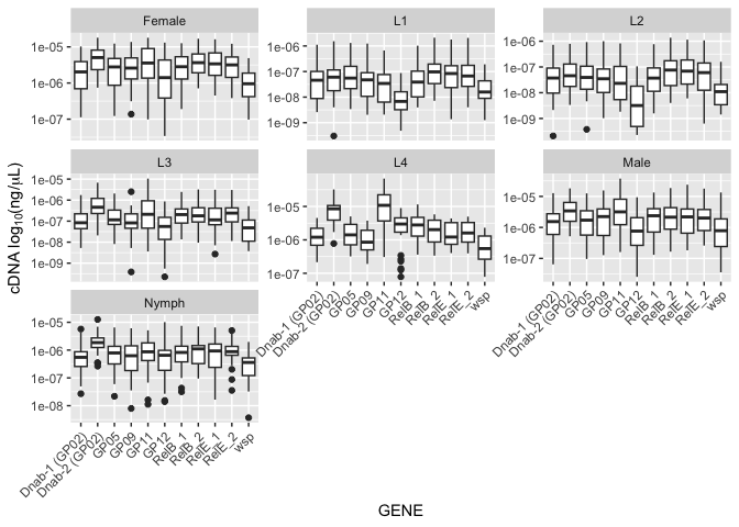
Boxplot intra-stage
ggplot(data_combined, aes(x = GENE, y = concentration)) +
  geom_boxplot() +
  facet_wrap(~Stage, scales = "free_y") +
  scale_y_log10() +
  theme(axis.text.x = element_text(angle = 45, hjust = 1))+
  labs(y = expression("cDNA " * log[10] * "(ng/" * mu * "L)"))