RosaBioinfo

Assembly of Isolate and wPipSLAB from short paired-end reads and related analyzes: taxonomical binning and read alignments

January 15, 2026

Maxime Mahout

• Notebook for Isolate and wPipSLAB assembly and read mapping to reference genomes
  • Assembly of Isolate and wPipSLAB
  • Mapping of Isolate reads on wPipPel
  • Mapping of Isolate reads on Isolate assembly
  • Mapping of Isolate reads on wPipSLAB and of SLAB reads on wPipSLAB
  • Detail of bowtie commands

Language: Bash

Notebook for Isolate and wPipSLAB assembly and read mapping to reference genomes

Here we describe the steps that were necessary to assemble the genome of the Isolate and the SLAB Wolbachia genome: wPipSLAB, as well as alignment to selected reference genomes.

The figure below summarizes the steps to get the assemblies of Isolate and wPipSLAB together with the mapping to reference genomes.

Note that profile coverage analyses and visualization - last step in the figure - will be described in the following notebooks.

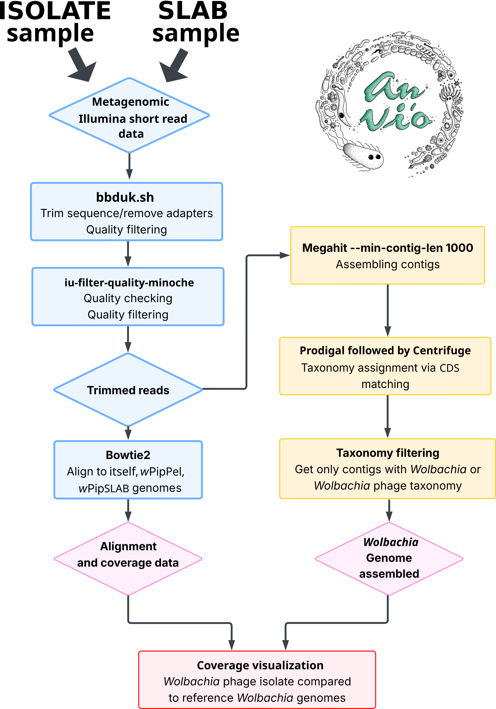
Assembly of Isolate and wPipSLAB

The steps taken for assembly of the Isolate genome and the new wPipSLAB reference are the same.

Of note, out of all of our SLAB samples (8 total samples of the same strain, data not shown), we selected the SLAB sample (namely SLAB002) that generated the longest assembled genome.

We used the standard metagenomic anvi’o assembly and binning pipeline.

Short paired-reads from Illumina of the samples are preliminarily trimmed of adapters using bbduk.

cat adapter_MGX.fa

>adapter_MGX
CTGTCTCTTATACACATCT

Steps apply for the Isolate short read samples as well as for the SLAB short read sample.

base_name=Isolate

base_name=SLAB

bbduk.sh in1="$real_r1" in2="$real_r2" \
        out1="${output_dir}/${base_name}_R1_001_trimmed.fastq.gz" \
        out2="${output_dir}/${base_name}_R2_001_trimmed.fastq.gz" \
        ref=adapter_MGX.fa \
        stats="${BASE_DIR}/Trimmed/stats/${base_name}_stats.txt" \
        ktrim=r k=19 mink=9 hdist=1 tpe tbo t=$SLURM_CPUS_PER_TASK

Now, here is the command for running the full anvi’o pipeline.

anvi-run-workflow -w metagenomics -c config_megahit_v8.json \
  --additional-params --keep-going --jobs 10 --jobscript jobscript_v8.sh \
  --rerun-incomplete --latency-wait 420

Where jobscript_v8.sh is a script that contains conda activation of anvio-8.

Interesting JSON lines of config_megahit_v8.json are described below.

First, this line is such that input_samples.txt describes the trimmed .fastq files of the samples in input.

    [...]
    "samples_txt": "input_samples.txt",
    [...]

Here is a version of “input_samples.txt” for the Isolate and here is a version for SLAB

Here are the lines defining how to quality check and filter reads (part of anvi’o tools).

    [...]
    "iu_filter_quality_minoche": {
        "run": true,
        "--ignore-deflines": true,
        "threads": 6
    },
    [...]

The following lines define how to filter out Culex quinquefasciatus reads.

    [...]
    "remove_short_reads_based_on_references": {
        "delimiter-for-iu-remove-ids-from-fastq": " ",
        "dont_remove_just_map": "",
        "references_for_removal_txt": "Cxq_masked_for_removal.txt",
        "threads": "6"
    },
    [...]

Below are the lines defining how to assemble all filtered reads into contigs with megahit, using a threshold of 1000 bp as minimum contig length.

    [...]
    "megahit": {
        "--min-contig-len": 1000,
        "--memory": 0.5,
        "threads": 4,
        "run": true,
        "--min-count": "",
        "--k-min": "",
        "--k-max": "",
        "--k-step": "",
        "--k-list": "",
        "--no-mercy": "",
        "--no-bubble": "",
        "--merge-level": "",
        "--prune-level": "",
        "--prune-depth": "",
        "--low-local-ratio": "",
        "--max-tip-len": "",
        "--no-local": "",
        "--kmin-1pass": "",
        "--presets": "meta-sensitive",
        "--mem-flag": "0",
        "--use-gpu": "",
        "--gpu-mem": "",
        "--keep-tmp-files": "",
        "--tmp-dir": "",
        "--continue": "",
        "--verbose": ""
    },
    [...]

Here are the lines defining how gene annotation (CDS) is performed - using prodigal as a backend.

    [...]
    "anvi_gen_contigs_database": {
        "--project-name": "{group}",
        "--description": "",
        "--skip-gene-calling": "",
        "--ignore-internal-stop-codons": "",
        "--skip-mindful-splitting": "",
        "--contigs-fasta": "",
        "--split-length": "",
        "--kmer-size": "",
        "--skip-predict-frame": "",
        "--prodigal-translation-table": "",
        "threads": ""
    },
    [...]

Below are the lines defining how to get taxonomy from CDS and the centrifuge p+h+v database.

    [...]
    "centrifuge": {
        "threads": 6,
        "run": true,
        "db": "/db/centrifuge/p+h+v"
    },
    [...]

Here are how reads are aligned to itself and possibly other genomes, giving coverage data useful for metagenomic binning.

    [...]
    "bowtie": {
        "additional_params": "--no-unal",
        "threads": 3
    },
    [...]

The actual bowtie command ran is the following:

bowtie2-align-s --wrapper basic-0 --threads 4 -x ./${sample}-contigs --passthrough -1 ./${sample}-FILTERED_R1.fastq.gz -2 ./${sample}-FILTERED_R2.fastq.gz > ${sample}.bam

Finally, taxonomic binning of this sample into Wolbachia contigs was performed by manual refining using the output from anvi’o (following automatic binning performed with CONCOCT).

anvi-refine -C CONCOCT_3 -b Wolbachia -c ./04_CONTIGS/${sample}-contigs.db -p ./07_MERGED/${sample}/PROFILE.db

Where ${sample} is either Isolate or SLAB.

Of note, we compensated lack of differential coverage data and incomplete taxonomy from centrifuge for the automatic binning of the Isolate sample by performing BLAST on all of our contigs and checking whether all contigs with BLAST hits were retrieved.

blastn \
    -query "$contigs_fasta_file" \
    -db "$NT_DB_LATEST" \
    -out "$output_file" \
    -outfmt "10 qseqid sseqid pident length mismatch gapopen qstart qend sstart send evalue bitscore stitle"

Mapping of Isolate reads on wPipPel

We start with a folder Data containing our trimmed Illumina reads of our Isolate.

ls Data/

Isolate1_R1_trimmed.fastq.gz  Isolate1_R2_trimmed.fastq.gz

We also need a genome that is a concatenation of wPipPel (GCF_000073005.1) and of pWCP (Reveillaud, Bordenstein et al, 2019) for future coverage analysis.

g="Genome/Ref_genome/wPipPel_Plasmid.fa"
echo $g

Genome/Ref_genome/wPipPel_Plasmid.fa

We then used the pipeline AliNE from Jacques Dainat https://github.com/Juke34/AliNe, without the trimming step.

./nextflow run Juke34/AliNe \
      -r v1.1.0 \
      -profile singularity \
      --trimming_fastp \
      --reads Data/ \
      --genome $g \
    --data_type DNA \
      --read_type short_paired \
      --aligner bowtie2 \
      --fastqc \
      --samtools_stats \
      -c nf.conf

The generated .bam is used for detailed coverage visualization in Supplementary Notebook 5 and Supplementary Notebook 6.

Mapping of Isolate reads on Isolate assembly

In addition, we mapped the Isolate reads onto the Isolate assembly.

This allows us to get coverage data for the Isolate for further analysis (Supplementary Notebook 7).

We can reuse AliNE with our trimmed reads but this time changing the reference genome.

Since this is a NextFlow pipeline and data is cached it won’t be recalculating quality checking.

All alignments are still performed with bowtie2.

g="Isolate.fasta"

./nextflow run Juke34/AliNe \
      -r v1.1.0 \
      -profile singularity \
      --reads Data/ \
      --genome $g \
    --data_type DNA \
      --read_type short_paired \
      --aligner bowtie2 \
      --fastqc \
      --samtools_stats \
      -c nf.conf

Mapping of Isolate reads on wPipSLAB and of SLAB reads on wPipSLAB

These last steps are required for the metapangenome layers of the pangenome analysis.

We use once again bowtie, however this time we use a pre-existing bowtie index of wPipSLAB and circumvent the use of the AliNE pipeline.

We describe the corresponding bowtie commands in Supplementary Notebook 3 and especially how to filter coverage on only Wolbachia contigs.

Detail of bowtie commands

All bowtie alignments ran in this study follow this specific command:

bowtie2-align-s --wrapper basic-0 --threads 4 -x ./${sample}-contigs --passthrough -1 ./${sample}-FILTERED_R1.fastq.gz -2 ./${sample}-FILTERED_R2.fastq.gz > ${sample}.bam

Note that these bowtie alignments do not generate any secondary alignments in the .bam file (unlike minimap2 for long reads) with the default parameters (-k is not set).

Consequently, if a read mapped perfectly (100% identity) to two positions, and both alignments got the same best score, only one is reported as primary while the others are not reported in the .bam file.

We double-checked this using the following command for displaying secondary alignments, ensuring it returned no output.

samtools view -f 256 Isolate1_FILTERED.bam

Also, as indicated in the Bowtie2 manual, in case of a tie for alignment score e.g. when mapping on repeated regions, alignments are randomly selected.

Read alignments were not filtered based on MAPQ values (we purposely kept all reads to specifically study coverage of genes within highly repetitive regions and retain ambiguity).